Download
1 / 35
370 likes | 566 Views
metric embeddings, graph expansion, and high-dimensional convex geometry. James R. Lee. Institute for Advanced Study. E(S, S). Given a graph G =( V,E) , and a subset S µ V , we denote. graph expansion and the sparsest cut. S. The edge expansion of G is the value. E(S, S).

E N D
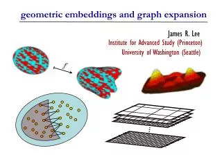
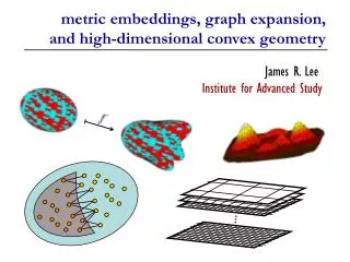
metric embeddings, graph expansion,and high-dimensional convex geometry James R. Lee Institute for Advanced Study
E(S, S) Given a graph G=(V,E), and a subset S µ V, we denote graph expansion and the sparsest cut S The edge expansion of G is the value
E(S, S) Given a graph G=(V,E), and a subset S µ V, we denote graph expansion and the sparsest cut S The edge expansion of G is the value
E(S, S) Given a graph G=(V,E), and a subset S µ V, we denote graph expansion and the sparsest cut S The edge expansion of G is the value Goal: Find the least-expanding cut in G (at least approximately).
There is a natural SDP-based approach: Spectral analysis (first try) geometric approach gap can be (n) even if G is an n-cycle! can be computed by a semi-definite program
SDP relaxation: geometric approach
SDP relaxation: geometric approach triangle inequality constraints: A distance function satisfying the above constraint is called a negative-type metric on V.
SDP relaxation: geometric approach triangle inequality constraints: impose a strange geometry on the solution space
geometric approach x · 90o y z Euclidean distance after t steps is at most √ t 1 triangle inequality constraints: impose a strange geometry on the solution space
Given two metric spaces (X,dX) and (Y,dY), an embedding of X into Y is a mapping f : X ! Y. embeddings and distortion The distortion of f is the smallest number D such that
Given two metric spaces (X,dX) and (Y,dY), an embedding of X into Y is a mapping f : X ! Y. embeddings and distortion The distortion of f is the smallest number D such that We will be concerned with the cases Y = L1 or Y = L2 (think of Y = Rn with the L1 or L2 norm) In this case, we write c1(X) or c2(X) for the smallest possible distortion necessary to embed X into L1 and L2, resp.
negative-type metrics (NEG), embeddings, L1, L2 the connection NEG metric (V,d) allow weights w(u,v) “sparsest cut” Integrality gap max c1(V,d) max distortion into L1 = =
So we just need to figure out a way to embed every NEG space into L1 with small distortion... embedding NEG spaces Problem: We don’t have strong L1-specific techniques. Let’s instead try to embed NEG spaces into L2 spaces (i.e. Euclidean spaces). This is actually stronger, since L2µ L1, but there is a natural barrier... Even the d-dimensional hypercube{0,1}d requires d1/2 = (log n)1/2 distortion to embed into a Euclidean space. GOAL: Prove that the hypercube is the “worst” NEG metric. Known: Every n-point NEG metric (V,d) has c2(V,d) = O(log n) [Bourgain] Conjecture: Every n-point NEG metric (V,d) has c2(V,d) = O(√log n)
embedding NEG spaces Conjecture: Every n-point NEG metric (V,d) has c2(V,d) = O(√log n) Implies O(√log n)-approximation for edge expansion (even SparsestCut), improving the previous O(log n) bound. [Leighton-Rao, Linial-London-Rabinovich, Aumann-Rabani] Also: Something provable to be gained from spectral approach! Thinking about the conjecture: Subsets of hypercubes{0,1}kprovide interesting NEG metrics. If you had to pick an n-point subset of some hypercube which is furthest from a Euclidean space, would you just choose {0,1}log n, or a sparse subset of some higher-dimensional cube?
The embedding comes in three steps average distortion (1) • Average distortion: Fighting concentration of measure • Want a non-expansive map f : X !Rn which sends a • “large fraction” of pairs far apart. f Rn Euclidean space NEG space
hypercube The embedding comes in three steps average distortion (1) • Average distortion: Fighting concentration of measure • Want a non-expansive map f : X !Rn which sends a • “large fraction” of pairs far apart. f Rn Every non-expansive map from {0,1}d into L2 maps most pairs to distance at most √d =√log n )average distance contracts by a √log n factor
d(A,B) ¸1/√log n The embedding comes in three steps average distortion (1) • Average distortion: Fighting concentration of measure • Want a non-expansive map f : X !Rn which sends a • “large fraction” of pairs far apart. |A| ¸n/5 f : X !R ¼1 |B| ¸n/5 B A 0 1/√log n
d(A,B) ¸1/√log n The embedding comes in three steps average distortion (1) • Average distortion: Fighting concentration of measure • Want a non-expansive map f : X !Rn which sends a • “large fraction” of pairs far apart. |A| ¸n/5 Theorem: Such sets A,B µ X always exist! [Arora-Rao-Vazirani] ¼1 |B| ¸n/5
2. Single-scale distortion Now we want a non-expansive map f : X !Rn which “handles” all the pairs x,y 2 X with d(x,y)¼1. single-scale distortion (2) A If we had a randomized procedure for generating A and B, then we could sample k = O(log n) random coordinates of the form x ! d(x, A), and handle every pair a constant fraction of the time (with high probability)... ¼1 B
Randomized version: Choosing A and B “at random” single-scale distortion (2) Rn • Choose a random (n-1)-hyperplane. A H want d(A0,B0)¸1/√log n B A0 B0 2.Prune the “exceptions.”
Randomized version: Choosing A and B “at random” single-scale distortion (2) Rn A Pruning)d(A,B) is large. The hard part is showing that |A|, |B| = (n) whp after the pruning! H B A0 B0 2.Prune the “exceptions.”
Randomized version: Choosing A and B “at random” single-scale distortion (2) Rn A Pruning)d(A,B) is large. The hard part is showing that |A|, |B| = (n) whp after the pruning! H [ARV]gives B [L] yields the optimal bound
Adversarial noise: A and B are not “random” enough single-scale distortion (2) Rn A A0, B0 would be great, but we are stuck with A,B After O(log n) iterations, every point is left un-pruned in at least ½ of the trials. [Chawla-Gupta-Racke] (multiplicative update): H • Give every point of X some weight. • 2. Make it harder to prune heavy points • 3. If a point is not pruned in some iteration, • half its weight. • 4. The adversary cannot keep pruning the • same point from the matching. B
3. Multi-scale distortion Finally, we want to take our analysis of “one scale” and get a low-distortion embedding. multi-scale distortion (3)
metric spaces have various scales multi-scale distortion (3)
3. Multi-scale distortion Need an embedding that handles all scales simultaneously. multi-scale distortion (3) So far, we know that if (X,d) is an n-point NEG metric, then...
3. Multi-scale distortion Known: Using some tricks, the number of “relevant” scales is only m = O(log n), so take the corresponding maps.... and just “concatenate” the coordinates and rescale: multi-scale distortion (3) Oops: The distortion of this map is only O(log n)!
[Krauthgamer-L-Mendel-Naor, LA, Arora-L-Naor, LB] multi-scale distortion (3) (measured descent, gluing lemmas, etc.) Basic moral:Not all scales are created equal. The local expansionof a metric space plays a central role. x Represents the “dimension” of X near x 2 X at scale R. Ratio small ) locality well-behaved. Key fact: X has only n points.
multi-scale distortion (3) The local expansionof a metric space plays a central role. x Represents the “dimension” of X near x 2 X at scale R. Ratio small ) locality well-behaved. Key fact: X has only n points.
multi-scale distortion (3) The local expansionof a metric space plays a central role. controls smoothness of bump functions (useful for gluing maps on a metric space) Represents the “dimension” of X near x 2 X at scale R. Ratio small ) locality well-behaved. controls size of “accurate” random samples Key fact: X has only n points.
multi-scale distortion (3) GLUING THEOREMS If such an ensemble exists, then X embeds in a Euclidean space with distortion... [KLMN, LA] (CGR) [ALN] [LB]
No hardness of approximation results are known for edge expansion under standard assumptions (e.g. P NP). lower bounds, hardness, and stability Recently, there have been hardness results proved using variants of Khot’s Unique Games Conjecture (UGC): [Khot-Vishnoi, Chawla-Krauthgamer-Kumar-Rabani-Sivakumar] And unconditional results about embeddings, and the integrality gap of the SDP: [Khot-Vishnoi, Krauthgamer-Rabani]
The analysis of all these lower bounds are based on isoperimetric stability results in graphs based on the discrete cube {0,1}d. lower bounds, hardness, and stability Classical fact: The cuts with minimal (S) are dimension cuts.
The analysis of all these lower bounds are based on isoperimetric stability results in graphs based on the discrete cube {0,1}d. lower bounds, hardness, and stability Stability version: Every near-optimal cut is “close” to a dimension cut. (much harder: uses discrete Fourier analysis)
open problems What is the right bound for embedding NEG metrics into L1? Does every planar graph metric embed into L1 with O(1) distortion? (Strongly related to “multi-scale gluing” for L1 embeddings) What about embedding edit distance into L1? (Applications to sketching, near-neighbor search, etc.)