Download

1 / 21
210 likes | 426 Views
A Comparison of Two MCMC Algorithms for Hierarchical Mixture Models. Russell Almond Florida State University College of Education Educational Psychology and Learning Systems ralmond@fsu.edu. Cognitive Basis. Multiple cognitive processes involved in writing

E N D
A Comparison of Two MCMC Algorithms for Hierarchical Mixture Models Russell Almond Florida State University College of Education Educational Psychology and Learning Systems ralmond@fsu.edu
Cognitive Basis • Multiple cognitive processes involved in writing • Different processes take different amounts of time • Transcription should be fast • Planning should be long • Certain event types should be more common than others
Multi-Process Model of Writing Deane (2009) Model of writing.
Mixture of Lognormals • Log Pause Time Yij = log(Xij) • Student (Level-2 unit) i=1,…,I • Pause (Level-1 unit) j=1,…,Ji • Zij ~ cat(pi1,…,piK) is an indicator for which of K components the jth pause for the ith student is in • Yij | Zij= k ~ N(mik,tik)
Mixture Model Component k Essay i tik Event j pi Zij Y*ijk mik yij
Mixture Model Problems • If pikis small for some k, then category disappears • If tikis small for some k, then category becomes degenerate • If mik=mik’ and tik=tik’then really only have K-1 categories
Labeling Components • If we swap the labels on component k and k’, the likelihood is identical • Likelihood is multimodal • Often put a restriction on the components: mi1 < mi2 < … < miK • Früthwirth-Schattner (2001) notes that when doing MCMC, better to let the chains run freely across the modes and sort out post-hoc • Sorting needs to be done before normal MCMC convergence tests, or parameter estimation
Key Question • How many components? • Theory: each component corresponds to a different combination of cognitive processes • Rare components might not be identifiable from data Hierarchical models which allow partial pooling across Level-2 (students) might help answer these questions
Hierarchical Mixture Model Component k t0k g0k Essay i tik Event j a pi Zij Y*ijk mik yij b0k m0k
Problems with hierarchical models • If g0k,b0k 0 we get complete pooling • If g0k,b0k∞ we get no pooling • Something similar happens with • Need prior distributions that bound us away from those values. • log(t0k), log(b0k), log(g0k) ~ N(0,1)
Two MCMC packages JAGS Stan Hamiltonian Monte Carlo Cycles take longer Less autocorrelation Cannot extend runs Must monitor all paramters • Random Walk Metropolis, or Gibbs sampling • Has a special proposal for normal mixtures • Can extend a run if insufficient length • Can select which parameters to monitor
Add redundant parameters to make MCMC faster • mik = m0k + qib0k • qi ~ N(0,1) • log(tik) = log(t0k) + hig0k • hi ~ N(0,1) • ak = a0kaN • a0 ~ Dirichlet(a0m) • aN ~ c2(2I)
Initial Values • Run EM on each student’s data set to get student-level (Level 1) parameters • If EM does not converge, set parameters to NA • Calculate cross-student (Level 2) as summary statistics of Level 1 parameters • Impute means for missing Level 1 parameters Repeat with subsets of the data for variety in multiple chains
Simulated Data Experiment • Run initial value routine on real data for K=2,3,4 • Generate data from the model using these parameters • Fit models with K’=2,3,4 to the data from true K=2,3,4 distributions in both JAGS (RWM) and Stan (HMC) • Results shown for K=2, K’=2
Results (Mostly K=2, K’=2) • All results (http://pluto.coe.fsu.edu/mcmc-hierMM) • Deviance/Log Posterior—Good Mixing • m01 (average mean of first component)—Slow mixing in JAGS • a01 (average probability of first component)—Poor convergence, switching in Stan • g01(s.d. of log precisions for first component)—Poor convergence, multiple modes?
Other Results • Convergence is still an issue • MCMC finds multiple modes, where EM (without restarts) typically finds only one • JAGS (RWM) was about 3 times faster than Stan (HMC) • Monte Carlo se in Stan about 5 times smaller (25 time larger effective sample size) • JAGS is still easier to use than Stan • Could not use WAIC statistic to recover K • Was the same for K’=2,3,4
Implication for Student Essays • Does not seem to recover “rare components” • Does not offer big advantage over simpler no pooling non-hierarchical model • Ignores serial dependence in data • Hidden Markov model might be better than straight mixture
Try it yourself • http://pluto.coe.fsu.edu/mcmc-hierMM/ • Complete source code (R, Stan, JAGS) including data generation • Sample data sets • Output from all of my test runs, including trace plots for all parameters • Slides from this talk.