Download

1 / 22
290 likes | 1.17k Views
Learn about Gaussian mixture models for clustering, parameter estimation, EM algorithm, responsibilities, and more with concrete examples and insights.

E N D
Speech and Image Processing UnitDepartment of Computer Science University of Joensuu, FINLAND Gaussian Mixture Models Clustering Methods: Part 8 Ville Hautamäki
Preliminaries • We assume that the dataset X has been generated by a parametric distribution p(X). • Estimation of the parameters of p is known as density estimation. • We consider Gaussian distribution. Figures taken from: http://research.microsoft.com/~cmbishop/PRML/
Typical parameters (1) • Mean(μ): average value of p(X), also called expectation. • Variance (σ): provides a measure of variability in p(X) around the mean.
Typical parameters (2) • Covariance: measures how much two variables vary together. • Covariance matrix: collection of covariances between all dimensions. • Diagonal of the covariance matrix contains the variances of each attribute.
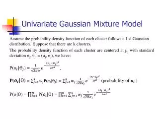
One-dimensional Gaussian • Parameters to be estimated are the mean (μ) and variance (σ)
Multivariate Gaussian (1) • In multivariate case we have covariance matrix instead of variance
Multivariate Gaussian (2) Diagonal Single Full covariance Complete data log likelihood:
Maximum Likelihood (ML) parameter estimation • Maximize the log likelihood formulation • Setting the gradient of the complete data log likelihood to zero we can find the closed form solution. • Which in the case of mean, is the sample average.
When one Gaussian is not enough • Real world datasets are rarely unimodal!
Mixtures of Gaussians (2) • In addition to mean and covariance parameters (now M times), we have mixing coefficients πk. Following properties hold for the mixing coefficients: It can be seen as the prior probability of the component k
Responsibilities (1) Complete data Incomplete data Responsibilities • Component labels (red, green and blue) cannot be observed. • We have to calculate approximations (responsibilities).
Responsibilities (2) • Responsibility describes, how probably observation vector x is from component k. • In clustering, responsibilities take values 0 and 1, and thus, it defines the hard partitioning.
Responsibilities (3) We can express the marginal density p(x) as: From this, we can find the responsibility of the kth component of x using Bayesian theorem:
Expectation Maximization (EM) • Goal: Maximize the log likelihood of the whole data • When responsibilities are calculated, we can maximize individually for the means, covariances and the mixing coefficients!
Exact update equations New mean estimates: Covariance estimates Mixing coefficient estimates
EM Algorithm • Initialize parameters • while not converged • E step: Calculate responsibilities. • M step: Estimate new parameters • Calculate log likelihood of the new parameters
Computational complexity • Hard clustering with MSE criterion is NP-complete. • Can we find optimal GMM in polynomial time? • Finding optimal GMM is in class NP
Some insights • In GMM we need to estimate the parameters, which all are real numbers • Number of parameters: M+M(D) + M(D(D-1)/2) • Hard clustering has no parameters, just set partitioning (remember optimality criteria!)
Some further insights (2) • Both optimization functions are mathematically rigorous! • Solutions minimizing MSE are always meaningful • Maximization of log likelihood might lead to singularity!