Download
1 / 30
370 likes | 863 Views
Comparing Two Means Dependent and Independent T-Tests. Class 14. Logic of Inferential Stats. Tony “Trout Eyes” Nullhype: “No fuggin way! I was at duh church rummage sale!”. Detective Althype: “Tony 'Trout Eyes' Nullhype was at the murder scene.”. Dataville Witness Reports

E N D
Comparing Two MeansDependent and Independent T-Tests Class 14
Logic of Inferential Stats Tony “Trout Eyes” Nullhype: “No fuggin way! I was at duh church rummage sale!” Detective Althype: “Tony 'Trout Eyes' Nullhype was at the murder scene.” Dataville Witness Reports Witness 1: Saw Tony at scene Witness 2: Saw Tony at scene Witness 3: Not sure Dataville Witness Reports Witness 1: Saw Tony at scene Witness 2: Saw Tony at scene Witness 3: Not sure Witness 4: Not sure Witness 5: Not sure Witness 6: Not sure Witness 7: Not sure Error
Logic of Inferential Stats Degree of Certainty All Observations 2 witnesses ID’d Tony = 0.66 confirmation rate 3 witnesses total 2 witness ID’d Tony = 0.29 confirmation rate 7 witnesses total
Generating Anxiety—Photos vs. Reality: Within Subjects and Between Subjects Designs Problem Statement: Are people as aroused by photos of threatening things as by the physical presence of threatening things? Hypothesis: Physical presence will arouse more anxiety than pictures. Expt’l Hypothesis: Seeing a real tarantula will arouse more anxiety than will spider photos.
WITHIN SUBJECTS DESIGN • All subjects see both spider pictures and real tarantula • Counter-balanced the order of presentation. Why? • DV: Anxiety after picture and after real tarantula Data (from spiderRM.sav) Subject Picture (anx. score) Real T (anx. score) 1 30 40 2 35 35 3 45 50 --- --- --- 12 50 39
Results: Anxiety Due to Pictures vs. Real Tarantula Yes Do the means LOOK different? Are they SIGNIFICANTLY DIFFERENT? Need t-test
WHY MUST WE LEARN FORMULAS? Don’t computers make stat formulas unnecessary 1. SPSS conducts most computations, error free 2. In the old days—team of 3-4 work all night to complete stat that SPSS does in .05 seconds. Fundamental formulas explain the logic of stats 1. Gives you more conceptual control over your work 2. Gives you more integrity as a researcher 3. Makes you more comfortable in psych forums
TODDLER FORMULA ) +( X (5) X (365 X3y) = Point: Knowing the formula without understanding concepts leads to impoverished understanding.
Logic of Testing Null Hypothesis Inferential Stats test the null hypothesis ("null hyp.") This means that test is designed to CONFIRM that the null hyp is true. In WITHIN GROUPS t-test (AKA "dependent" t-test) null hyp. is that responses in Cond. A and in Cond. B come from same population of responses. Null hyp.: Cond A and Cond B DON'T differ. In BETWEEN GROUPS t-test (AKA "independent" t-test) null hyp. is that responses from Group A and from Group B DON’T differ. If tests do not confirm the null hyp, then must accept ALT. HYPE. Alt. hyp. within-groups: Cond A differs from Cond B Alt. hyp. between-groups Group A differs from Group B
Null Hyp. and Alt. Hyp in Pictures vs. Reality Study Within groups design: Cond. A (all subjs. see photos), then Cond. B (all subs. see actual tarantula) Anxiety ratings Null hyp? No differences between seeing photos (Cond A) and seeing real T (Cond B) Alt. hyp? There is a difference between seeing photos (Cond A) and seeing real T (Cond B)
T-Test as Measure of Difference Between Two Means 1. Two data samples—do means of each sample differ significantly? 2. Do samples represent same underlying population (null hyp: small diffs) or two distinct populations (alt. hyp: big diffs)? 3. Compare diff. between sample means to diff. we’d expect if null hyp is true 4. Use Standard Error (SE) to gauge variability btwn means. a. If SE small & null hyp. true, sample diffs should be smaller b. If SE big & null hyp. true, sample diffs. should be larger 5. If sample means differ much more than SE, then either: a. Diff. reflects improbable but true random difference w/n true pop. b. Diff. indicates that samples reflect two distinct true populations. 6. Larger diffs. Between sample means, relative to SE, support alt. hyp. 7. All these points relate to both Dependent and Independent t-tests
Logic of T-Test expected difference between population means (if null hyp. is true) observed difference between sample means − t = SE of differencebetween sample means Note: Logic the same for Dependent and Independent t-tests. However, the specific formulas differ.
Mean Difference Relative to SE (overlap) Small: Null Hyp. Supported Mean Difference Relative to SE (overlap) Large: Alternative Hyp. Supported
SD: The Standard Error of Differences Between Means Sampling Distribution: The spread of many sample means around a true mean. SE: The average amount that sample means vary around the true mean. SE = Std. Deviation of sample means. Formula for SE: SE = s/√n, when n > 30 If sample N > 30 the sampling distribution should be normal. Mean of sampling distribution = true mean. SD = Average amount Var. 1 mean differs from Var. 2 mean in Sample 1, then in Sample 2, then in Sample 3, ---- then in Sample N Note: SD is differently computed in Between-subs. designs.
SD: The Standard Error of Differences Between Means TARANTULA PICTURE D MEAN MEAN (T mean – P mean) Study 1 6 3 3 Study 2 5 3 2 Study 3 4 2 2 Study 4 5 3 2 . Ave. 2.25
SD: The Standard Error of Differences Between Means TARANT.PICT.D D - D (D-D)2 Sub. 1 6 3 3 -. 75 .56 Sub. 2 5 3 2 .25 .07 Sub. 3 4 2 2 .25 .07 Sub. 4 5 3 2 .25 .07 X Tarant = 5 X Pic = 2.75 D = 2.25 Σ (D-D)2 = .77 SD2 = Sum (D -D)2 / N - 1; = .77 / 3 = .26 SD = √SD2 = √.26 = .51 SE of D = σD = SD / √N = .51 / √4 = .51 / 2 = .255 t = D / SE of D = 2.25 / .255 = 8.823
Understanding SD and Experiment Power Power of Experiment: Ability of expt. to detect actual differences. Small SD indicates that average difference between pairs of variable means should be large or small, if null hyp true? Small Small SD will therefore increase or decrease our chance of confirming experimental prediction? Increase it.
Assumptions of Dependent T-Test 1. Samples are normally distributed 2. Data measured at interval level (not ordinal or categorical)
D− μD Conceptual Formula for Dependent Samples T-Test Experimental Effect t = = Random Variation sD/ √N D = Average difference between mean Var. 1 – mean Var. 2. It represents systematic variation, aka experimental effect. μD = Expected difference in true population = 0It represents random variation, aka the the null effect. sD/ √N = Estimated standard error of differences between all potential sample means. It represents the likely random variation between means.
Dependent (w/n subs) T-Test SPSS Output t = expt. effect / error t = X / SE t = -7 / 2.83 = -2.473 Note: SE = SD / √n 2.83 = 9.807 / √12 Mean = mean diff pic anx - real anx. = 40 - 47 = - 7
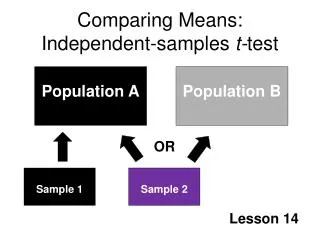
Independent (between-subjects) t-test • Subjects see either spider pictures OR real tarantula • Counter-balancing less critical (but still important). Why? • DV: Anxiety after picture OR after real tarantula Data (from spiderBG.sav) Subject Condition Anxiety 1 1 30 2 2 35 3 1 45 22 2 50 23 1 60 24 2 39
Assumptions of Independent T-Test DEPENDENT T-TEST 1. Samples are normally distributed 2. Data measured at least at interval level (not ordinal or categorical) INDEPENDENT T-TESTSALSO ASSUME 3. Homogeneity of variance 4. Scores are independent (b/c come from diff. people).
Logic of Independent Samples T-Test (Same as Dependent T-Test) expected difference between population means (if null hyp. is true) observed difference between sample means − t = SE of difference between sample means Note: SE of difference of sample means in independent t test differs from SE in dependent samples t-test
Conceptual Formula for Independent Samples T-Test (X1 − X2) − (μ1−μ2) Experimental Effect t = = Est. of SE Random Variation (X1 − X2) = Diffs. btwn. samples It represents systematic variation, aka experimental effect. (μ1 − μ2) = Expected difference in true populations = 0It represents random variation, aka the the null effect. Estimated standard error of differences between all potential sample means. It represents the likely random variation between means.
X1− X2 √ 2 sp sp + Computational Formulas for Independent Samples T-Tests t = X1− X2 t = ( ) √ 2 2 s1 s2 2 + N1 N2 n1 n2 When N1 = N2 When N1 ≠ N2 Weighted average of each groups SE 2 2 sp (n1 -1)s1 + (n2 -1)s2 2 = = n1 + n2− 2
Independent (between subjects) T-Test SPSS Output t = expt. effect / error t = (X1 − X2) / SE t = -7 / 4.16 = - 1.68
Dependent (within subjects) T-Test SPSS Output t = expt. effect / error t = X / SE t = -7 / 2.83 = -2.473 Note: SE = SD / √n 2.83 = 9.807 / √12 Mean = mean diff pic anx - real anx. = 40 - 47 = - 7
Dependent T-Test is Significant; Independent T-Test Not Significant. A Tale of Two Variances Independent T -Test Dependent T-Test SE = 4.16 SE = 2.83