Download
1 / 26
260 likes | 434 Views
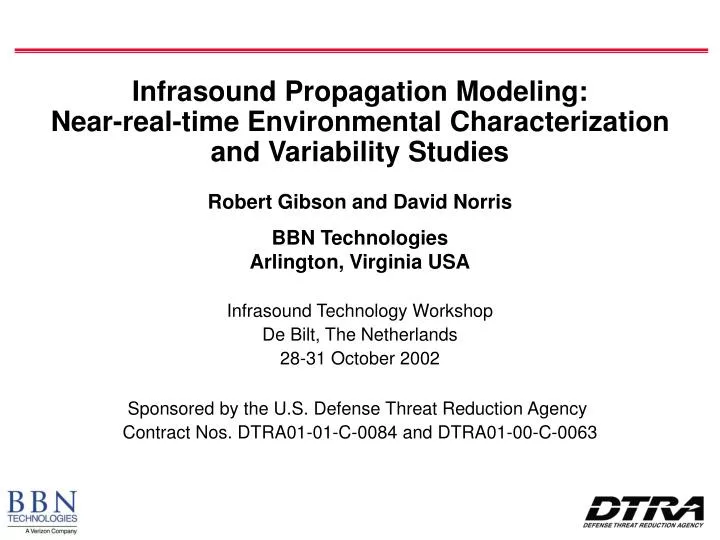
Infrasound Propagation Modeling: Near-real-time Environmental Characterization and Variability Studies. Robert Gibson and David Norris BBN Technologies Arlington, Virginia USA Infrasound Technology Workshop De Bilt, The Netherlands 28-31 October 2002

E N D
Infrasound Propagation Modeling: Near-real-time Environmental Characterization and Variability Studies Robert Gibson and David Norris BBN Technologies Arlington, Virginia USA Infrasound Technology Workshop De Bilt, The Netherlands 28-31 October 2002 Sponsored by the U.S. Defense Threat Reduction Agency Contract Nos. DTRA01-01-C-0084 and DTRA01-00-C-0063
InfraMAP Objectives • Integrate the software tools needed to perform infrasound propagation modeling. • Define the state of the atmosphere (temperature, wind) as required for input to propagation models. • Predict phases (travel times, bearings, amplitudes) from atmospheric explosions as measured by infrasound sensors. • Apply tools to support nuclear explosion monitoring R&D and resolve operational issues: • environmental variability and propagation sensitivity • prediction of localization area of uncertainty and detection performance • performance model of an infrasound network
Environmental Analysis • Empirical characterizations are built-in • User-defined profiles can be imported • View Environment functions via GUI • Seamless integration with propagation models
Motivation for Current Work • Evaluate methods to improve infrasound localization and phase identification. • Apply advanced modeling to investigate improvements to operational processing. • Recommendations from the 2001 Infrasound Technology Workshop: • “Routine processing needs to incorporate more precise estimates of the atmospheric state.” • “Support integration of required environmental information for modeling … leading to final goal of an operational full modeling capability.” • Support infrasound R&D community by maintaining InfraMAP as user-friendly modeling tool kit.
InfraMAP Software Schematic Azimuth Deviation Travel Time Elevation Angle Attenuation Synthetic Waveform from modes Variability Statistics Propagation Environment GUI GUI Date Time Latitude Longitude Altitude Environmental Characterization • MSIS-90 • HWM-93 • User-defined profile • Environmental Variability Propagation Modeling Near-Real-Time Updates • NRL-MSIS-00 • Next-Generation HWM • Ground-to-Space Assimilation Model Parameters Source Localization Area of Uncertainty Network Performance Synthetic Phases from rays • Ray Tracing • Normal Mode • Parabolic Equation • Model-based assimilation • In-situ measurements • Solar/Magnetic parameters Network Performance Modeling GUI GUI
Approach and Applications • Incorporate updated atmospheric characterizations • Evaluate best available sources • Integrate with propagation models and user-interfaces • Conduct sensitivity studies • Apply propagation statistics to localization problem • Model bias and variance • Investigate techniques to refine source localization • Predict uncertainty and network performance • Model observed infrasound events • Obtain ground truth source location • Compare model results with observations • Assess quality of atmospheric characterization
Numerical Weather Prediction • Physics-based models that assimilate data from many sources • Grids produced 2 to 4 times per day by various organizations • Interpolation (3-d) and merging (in altitude) are required • Example: NOGAPS from US Navy’s Fleet Numerical Meteorology and Oceanography Center (FNMOC) • Navy Operational Global Atmospheric Prediction System • NOGAPS grid is nonuniform in altitude. Highest available level is typically at 10 mb atmospheric pressure • Figures at right show temperatures along a slice of the atmosphere at fixed longitude (60 W) • Top: MSIS-00 • Bottom: NOGAPS
NOGAPS Gridded Data Example Left: Zonal Wind Right: Meridional Wind Top: HWM-93. Bottom: NOGAPS
Gridded Data Incorporation HWM MSIS Transition layer Derivatives at endpoints Spline through NOGAPS points • Issue: Ray models are highly sensitive to sharp changes in sound speed. Therefore, estimation approach must avoid introducing gradient variability not inherent to the data set. • Approach: A cubic spline algorithm is being developed to interpolate gridded data and to merge grid with empirical models. • Cubic spline interpolation provides smooth 1st derivative and continuous 2nd derivative, assuring compatibility with ray modeling. Temperature (T) Zonal (U) Meridional (V)
Range Dependence • Below: Integrated winds for ten latitude cells at a fixed longitude (60 W) • White lines indicate 10 km transition zone between NOGAPS and HWM Zonal (U) Meridional (V)
Ray Tracing Example IS41 NOGAPS grid subset • Search for stratospheric eigenrays over 1000 km eastward path in S. Am. • IS41, Villa Florida, Paraguay. 25 July 2002, 0:00 UT. • Left: MSIS/HWM Right: NOGAPS 3-d grid In this case, use of near-real-time grid reduces stratospheric turning height and introduces additional duct below 10 km.
Environment for Example Case Sample profiles from modeled scenario: NOGAPS and 10 km transition layer in blue,MSIS/HWM in red
IS26 IS10 NVIAR DLIAR IS57 Source IS59 Baseline localization Ground Truth Pacific Bolide: Baseline Localization • Event • Bolide 23 Apr 2001 • Ground Truth determined using satellites • Baseline localization from CMR study of detections at 6 stations using seasonal velocity model • Brown and Gault, CMR Tech Report CMR-01/09, 2001 • Key features • MLE algorithm using both measured back azimuths and arrival times • Signal velocities estimated from season-based velocity model • Large travel time variance specified to account for ray class (Stratospheric, Thermospheric) uncertainty • No correction for azimuthal deviation due to horizontal translation/refraction of ray paths • Baseline localization • Ground truth on edge of AOU • Ground truth/localization mismatch: 138 km • AOU: 85,400 sq km
Model-Enhanced Approach • Baseline localization used as initial data point for modeling. • Ray traces computed to identify ray class (stratospheric or thermospheric) that is most consistent with baseline localization. • For identified ray class, mean signal velocity and azimuthal deviation computed and used in new localization. • Atmospheric variability accounted for by using spectral gravity wave model. Propagation variability due to environment found by performing Monte Carlo simulation in which rays are propagated through perturbed realizations of atmosphere. • Total uncertainties (travel time variance, azimuth variance) computed by combining ray variability within ray class, propagation variability due to environment, and measurement error: • Azimuthal variance dominated by measurement resolution • Travel time variance dominated by ray variability within ray class • Model-enhanced localization found from same baseline MLE algorithm but using: • New signal velocity estimates • Back azimuth measurements corrected by azimuthal deviation estimates • New estimates for variances of travel time and azimuth • Ray classification details ->
Thermospheric rays Diffracted Stratospheric rays IS59 Ray Classification • Reverse propagate fan of rays from receivers to baseline localization • Group rays in classes: Thermospheric, Diffracted Stratospheric • Diffracted Stratospheric ray class • Rays that are trapped in elevated duct 10 km above ground • Assume ray reaches receiver through diffraction/scatter of energy from 10 km height IS59 • Ray classification achieved by comparing mean Signal Velocity and Azimuthal Deviation within a ray class with that found using baseline localization IS59 example: Signal velocity used in baseline localization well modeled by mean value of diffracted stratospheric rays
Ray Classification Observations Ray class IDs, and associated mean and standard deviations • Signal velocity found to be better discriminator than azimuthal deviation in this case • Classification approach did not clearly indicate a dominant ray class in all cases • More research needs to be done • Ray classification over multiple iterations of source localizations • Use of additional discriminators (phase arrival envelope, amplitude, etc.)
Model-Enhanced Localization • New localization found using same MLE algorithm as was used for baseline localization but with: • New signal velocity estimates • Back azimuth measurements corrected by azimuthal deviation • New summed estimates for variances of travel time and azimuth • Key improvements • More accurate signal velocity estimates • Smaller uncertainty in travel time • Model-enhanced Localization • Ground truth again on edge of AOU • Ground truth/localization mismatch: 85 km • AOU: 9834 sq km Baseline localization Model-enhanced localization Ground Truth Final localization accuracy increased by 38% with AOU decreased by 88%
Explosive eruption 2001-July-29 ~0600 GMT Observed at Deelen, NL and elsewhere in Europe Ground truth from Deelen: ~1750 km 152.4 degrees Observed azimuth of arrival 155-156 degrees ~ +2.5 to +3.5 degrees of azimuth deviation Data analysis by L. Evers (KNMI) Predicted azimuth using InfraMAP 156.4 degrees; +4 degrees deviation Thermospheric paths Using empirical atmospheric models Little change using NWP model up to 35 km Case Study: Etna Eruption
Space Shuttle Modeling Approach • Source of infrasound is not impulsive, but continuous and moving • Approximate moving source by modeling a series of discrete events, each with appropriate time delay • Use 3-D ray tracing to find eigenrays from points on launch trajectory to infrasound array • Orbiter • Solid rocket boosters (SRB) • Determine arrival time and azimuth for each eigenray Example of eigenrays from one point on trajectory to array location
Conclusions • Software models are being successfully used to predict travel time and bearing biases for atmospheric infrasound. • Empirical atmospheric modeling (climatology) is adequate for many scenarios, but not all. • Software development is underway to incorporate output of numerical weather prediction models into InfraMAP. • Propagation statistics are being incorporated into localization, AOU, and network performance predictions. • Rocket launches are a promising source of ongoing calibration data to validate environmental characterizations.