Download
1 / 23
310 likes | 595 Views
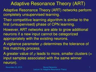
Adaptive Resonance Theory (ART). Adaptive Resonance Theory (ART) networks perform completely unsupervised learning. Their competitive learning algorithm is similar to the first (unsupervised) phase of CPN learning.

E N D
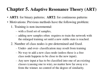
Adaptive Resonance Theory (ART) Adaptive Resonance Theory (ART) networks perform completely unsupervised learning. Their competitive learning algorithm is similar to the first (unsupervised) phase of CPN learning. However, ART networks are able to grow additional neurons if a new input cannot be categorized appropriately with the existing neurons. A vigilance parameter determines the tolerance of this matching process. A greater value of leads to more, smaller clusters (= input samples associated with the same winner neuron). Neural Networks Lecture 19: Adaptive Resonance Theory
Adaptive Resonance Theory (ART) ART networks consist of an input layer and an output layer. We will only discuss ART-1 networks, which receive binary input vectors. Bottom-up weights are used to determine output-layer candidates that may best match the current input. Top-down weights represent the “prototype” for the cluster defined by each output neuron. A close match between input and prototype is necessary for categorizing the input. Finding this match can require multiple signal exchanges between the two layers in both directions until “resonance” is established or a new neuron is added. Neural Networks Lecture 19: Adaptive Resonance Theory
Adaptive Resonance Theory (ART) ART networks tackle the stability-plasticity dilemma: Plasticity: They can always adapt to unknown inputs (by creating a new cluster with a new weight vector) if the given input cannot be classified by existing clusters. Stability: Existing clusters are not deleted by the introduction of new inputs (new clusters will just be created in addition to the old ones). Problem: Clusters are of fixed size, depending on . Neural Networks Lecture 19: Adaptive Resonance Theory
1 2 3 1 2 3 4 The ART-1 Network Output layer with inhibitory connections Input layer Neural Networks Lecture 19: Adaptive Resonance Theory
Initialize each top-down weight tl,j(0) = 1; Initialize bottom-up weight bj,l(0) = ; C. While the network has not stabilized, do Present a randomly chosen pattern x = (x1,…,xn) for learning Let the active set A contain all nodes; calculate yj = bj,1 x1 +…+bj,nxnfor each nodejA; 3. Repeat Let j* be a node in A with largest yj, with ties being broken arbitrarily; Compute s* = (s*1,…,s*n ) where s*l = tl,j* xl; Compare similarity between s* and x with the given vigilance parameter r: if<rthen remove j* from set A else associate x with node j* and update weights: bj*l (new) = tl,j*(new) = UntilA is empty or x has been associated with some node j 4. If A is empty, then create new node whose weight vector coincides with current input pattern x; end-while Neural Networks Lecture 19: Adaptive Resonance Theory
ART Example Computation For this example, let us assume that we have an ART-1 network with 7 input neurons (n = 7) and initially one output neuron (n = 1). Our input vectors are {(1, 1, 0, 0, 0, 0, 1), (0, 0, 1, 1, 1, 1, 0), (1, 0, 1, 1, 1, 1, 0), (0, 0, 0, 1, 1, 1, 0), (1, 1, 0, 1, 1, 1, 0)} and the vigilance parameter = 0.7. Initially, all top-down weights are set to tl,1(0) = 1, and all bottom-up weights are set to b1,l(0) = 1/8. Neural Networks Lecture 19: Adaptive Resonance Theory
ART Example Computation For the first input vector, (1, 1, 0, 0, 0, 0, 1), we get: Clearly, y1 is the winner (there are no competitors). Since we have: the vigilance condition is satisfied and we get the following new weights: Neural Networks Lecture 19: Adaptive Resonance Theory
ART Example Computation Also, we have: We can express the updated weights as matrices: Now we have finished the first learning step and proceed by presenting the next input vector. Neural Networks Lecture 19: Adaptive Resonance Theory
ART Example Computation For the second input vector, (0, 0, 1, 1, 1, 1, 0), we get: Of course, y1 is still the winner. However, this time we do not reach the vigilance threshold: This means that we have to generate a second node in the output layer that represents the current input. Therefore, the top-down weights of the new node will be identical to the current input vector. Neural Networks Lecture 19: Adaptive Resonance Theory
ART Example Computation The new unit’s bottom-up weights are set to zero in the positions where the input has zeroes as well. The remaining weights are set to:1/(0.5 + 0 + 0 + 1 + 1 + 1 + 1 + 0) This gives us the following updated weight matrices: Neural Networks Lecture 19: Adaptive Resonance Theory
ART Example Computation For the third input vector, (1, 0, 1, 1, 1, 1, 0), we have: Here, y2 is the clear winner. This time we exceed the vigilance threshold again: Therefore, we adapt the second node’s weights. Each top-down weight is multiplied by the corresponding element of the current input. Neural Networks Lecture 19: Adaptive Resonance Theory
ART Example Computation The new unit’s bottom-up weights are set to the top-down weights divided by (0.5 + 0 + 0 + 1 + 1 + 1 + 1 + 0). It turns out that, in the current case, these updates do not result in any weight changes at all: Neural Networks Lecture 19: Adaptive Resonance Theory
ART Example Computation For the fourth input vector, (0, 0, 0, 1, 1, 1, 0), it is: Again, y2 is the winner. The vigilance test succeeds once again: Therefore, we adapt the second node’s weights. As usual, each top-down weight is multiplied by the corresponding element of the current input. Neural Networks Lecture 19: Adaptive Resonance Theory
ART Example Computation The new unit’s bottom-up weights are set to the top-down weights divided by (0.5 + 0 + 0 + 0 + 1 + 1 + 1 + 0). This gives us the following new weight matrices: Neural Networks Lecture 19: Adaptive Resonance Theory
ART Example Computation Finally, the fifth input vector, (1, 1, 0, 1, 1, 1, 0), gives us: Once again, y2 is the winner. The vigilance test fails this time: This means that the active set A is reduced to contain only the first node, which becomes the uncontested winner. Neural Networks Lecture 19: Adaptive Resonance Theory
ART Example Computation The vigilance test fails for the first unit as well: We thus have to create a third output neuron, which gives us the following new weight matrices: Neural Networks Lecture 19: Adaptive Resonance Theory
ART Example Computation In the second epoch, the first input vector, (1, 1, 0, 0, 0, 0, 1), gives us: Here, y1 is the winner, and the vigilance test succeeds: Since the current input is identical to the winner’s top-down weights, no weight update happens. Neural Networks Lecture 19: Adaptive Resonance Theory
ART Example Computation The second input vector, (0, 0, 1, 1, 1, 1, 0), results in: Now y2 is the winner, and the vigilance test succeeds: Again, because the current input is identical to the winner’s top-down weights, no weight update occurs. Neural Networks Lecture 19: Adaptive Resonance Theory
ART Example Computation The third input vector, (1, 0, 1, 1, 1, 1, 0), give us: Once again, y2 is the winner, but this time the vigilance test fails: This means that the active set is reduced to A = {1, 3}. Since y3 > y1, the third node is the new winner. Neural Networks Lecture 19: Adaptive Resonance Theory
ART Example Computation The third node does satisfy the vigilance threshold: This gives us the following updated weight matrices: Neural Networks Lecture 19: Adaptive Resonance Theory
ART Example Computation For the fourth vector, (0, 0, 0, 1, 1, 1, 0), the second node wins, passes the vigilance test, but no weight changes occur. The fifth vector, (1, 1, 0, 1, 1, 1, 0), makes the second unit win, which fails the vigilance test. The new winner is the third output neuron, which passes the vigilance test but does not lead to any weight modifications. Further presentation of the five sample vectors do not lead to any weight changes; the network has thus stabilized. Neural Networks Lecture 19: Adaptive Resonance Theory
Adaptive Resonance Theory Illustration of the categories (or clusters) in input space formed by ART networks. Notice that increasing leads to narrower cones and not to wider ones as suggested by the figure. Neural Networks Lecture 19: Adaptive Resonance Theory
Adaptive Resonance Theory A problem with ART-1 is the need to determine the vigilance parameter for a given problem, which can be tricky. Furthermore, ART-1 always builds clusters of the same size, regardless of the distribution of samples in the input space. Nevertheless, ART is one of the most important and successful attempts at simulating incremental learning in biological systems. Neural Networks Lecture 19: Adaptive Resonance Theory