Plane Wave Basis Boundary Elements and Finite Elements for Wave Scattering Problems

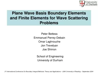
1. Plane Wave Basis Boundary Elements and Finite Elements for Wave Scattering Problems Peter Bettess Emmanuel Perrey-Debain Omar Laghrouche Jon Trevelyan Joe Shirron School of Engineering University of Durham

2. Peter Bettess University of Durham Omar Laghrouche Heriot-Watt University, Edinburgh Emmanuel Perrey-Debain UMIST, Manchester Joe Shirron Metron, Inc, Virginia, U.S.A. Jon Trevelyan University of Durham ResearchersCurrent Affiliations

4. Durham Cathedral

7. I do not propose to survey the extensive literature. Two recent volumes give an introduction to the field. Background

13. Presentation topics • Introduction • Mathematical formulation for the 2D Helmholtz problem • Conditioning and Singular Value Decomposition • Numerical results, convergence and accuracy analysis • The 3D Helmholtz problem • The 2D elastodynamic problem • Conclusions and prospects

14. 1. Introduction Motivation

15. 1. Introduction What about the use of plane waves ? • Volume discretization scheme • Partition of Unity Method (Babuška and Melenk 1997, Laghrouche et al. 2002) • Least-Squares (Stojek 1998, Monk and Wang 1999) • Ultra Weak Formulation (Cessenat and Després 1998, Huttunen et al. 2002) • Discontinuous Enrichment Method (Farhat et al. 2002) • Surface discretization scheme • Micro-local discretization (de La Bourdonnaye 1994) • Wave Boundary Elements (Perrey-Debain et al. 2002, 2003) • Specific use of plane waves for high frequency scattering problems in • (Abboud et al. 1995, Bruno et al. 2003, Chandler-Wilde et al. 2003)

16. 2. Mathematical formulation… Problem: we consider a two dimensional obstacle of general shape  in an infinite propagative medium  impinged by a incident time-harmonic wave inc We seek the potential  in  as the solution of the Helmholtz equation: The integral formulation reads (1) where is the free-space Green function

17. ) ( 2. Mathematical formulation… Geometry Boundary conditions Incident wave field

18. 2. Mathematical formulation… Plane wave basis function We can write the solution of (1) in the compact form: where the Q plane waves propagate in various directions evenly distributed over the unit circle: Note: Continuity requirement leads to N=2nQ degrees of freedom

19. 2. Mathematical formulation… Numerical implementation Matrix system Plane wave interpolation matrix (sparse) Boundary matrix (full) Plane wave coefficients

20. 3. Conditioning and SVD Ideal case, plane wave interpolation on the real line FFT matrix when =2 The interpolation matrix reads where  denotes the discretization level (DOF per wavelength) and  is the sampling rate Computed case, we define the average discretization level by

21. 3. Conditioning and SVD Condition number (2-norm) vs discretization level  Ideal case Computed (: unit circle, =0, N=2nQ=64) FFT matrix

22. 3. Conditioning and SVD

23. 3. Conditioning and SVD

24. 4. Numerical results, convergence and accuracy analysis Consider the unit circle and a regular subdivision with and Then the analytical solution can be expanded as where

25. The QR solver is used for all except these two most ill-conditioned cases for which SVD is used with =10-12 4. Numerical results, convergence and accuracy analysis Test case: scattering by the unit circle with =100 and =-100i Quadratic Q=5 Q=10 Q=25

26. 4. Numerical results, convergence and accuracy analysis 1 2 1 2

27. 4. Numerical results, convergence and accuracy analysis 

28. 4. Numerical results, convergence and accuracy analysis Water wave-structure interaction (a=1.7). Discretization: n=2 elements and Q=16 wave directions Incident plane wave at 45o

29. 4. Numerical results, convergence and accuracy analysis Test case: scattering by a 50-width boomerang-shaped obstacle

30. 5. The 3D Helmholtz problem Problem statement and notation

31. 5. The 3D Helmholtz problem Finite element discretization Plane wave basis

32. 5. The 3D Helmholtz problem 8 triangular patches and 6 vertices are sufficient to describe the scatterer

33. 5. The 3D Helmholtz problem Scattering of a vertical plane wave by the unit sphere Finite element formulation Integral formulation (From O. Laghrouche)

34. 5. The 3D Helmholtz problem Scattering by a thin plate (=3.1) Re () (0,0,1) (1,0,1)/2 Shadow zone Iluminated zone

35. 5. The 3D Helmholtz problem Ellipsoid (20 x 4 x 4) – Far Field Pattern Convergence reached with N=1308 variables (=2.65)

36. 5. The 3D Helmholtz problem Distorted scatterer geometry (=2.9) || (0,0,1) (1,0,1)/2 (1,0,0)

37. 6. The 2D elastodynamic problem

38. 6. The 2D elastodynamic problem

39. 6. The 2D elastodynamic problem

40. 6. The 2D elastodynamic problem

41. 6. The 2D elastodynamic problem

42. 6. The 2D elastodynamic problem

43. 6. The 2D elastodynamic problem

44. 6. The 2D elastodynamic problem

45. 13. Conclusions and prospects • Positive aspects of the `wave boundary element method’ • Not restricted to a specific problem • Possible extension of the method to other wave problems • Only approximately 2.5 - 3 variables per wavelength are required • Can provide extremely accurate results • Drawbacks • Ill-conditioned matrices require careful integration procedure and the use of appropriate solvers like truncated SVD • Matrix coefficients evaluation is time-consuming • In Prospects • Speed up the numerical integration • Investigate the Galerkin formulation for BE • Find good preconditioners for iterative algorithms

46. 7. Finite elements for Short Wave Modelling Motivation: Solve short wave problems where L/ >> 1 Applications: geophysics (hydro-carbon exploration), coastal and earthquake waves, acoustic and electromagnetic scattering, …

47. Objective - Applications Conventional methods Ray theory & SEA ? frequency Aim: Develop wave finite elements capable of containing many wavelengths per nodal spacing Applications: Problems involving large boundaries and/or short wavelengths

48. 9. Formulation of the plane wave finite elements Conventional Plane wave basis Idea: Include the wave character of the wave field in the element formulation

49. 10. Wave scattering in 2D Potential around the cylinder, ka=24

50. Reduction in dof ~ 1/15 10. Wave scattering in 2D