Community Ecology BDC331
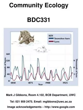
Community Ecology BDC331. Mark J Gibbons, Room 4.102, BCB Department, UWC Tel: 021 959 2475. Email: mgibbons@uwc.ac.za. Image acknowledgements – http://www.google.com. 1 – physically defined communities. Assemblages of species found in a particular place or habitat.

Community Ecology BDC331
E N D
Presentation Transcript
Community Ecology BDC331 Mark J Gibbons, Room 4.102, BCB Department, UWC Tel: 021 959 2475. Email: mgibbons@uwc.ac.za Image acknowledgements – http://www.google.com
1 – physically defined communities Assemblages of species found in a particular place or habitat How to Identify Communities ARTIFICIAL?
Great Smoky Mountains Tennessee Topographic distributions of the characteristic dominant tree species of the Great Smokey Mountains, Tennessee, on an idealized west-facing mountain and valley BG, beech gap; CF, cove forest; F, Fraser fir forest; GB, grassy bald; H, hemlock forest; HB, heath bald; OCF, chestnut oak-chestnut forest; OCH, chestnut oak-chestnut heath; OH, oak-hickory; P, pine forest & heath; ROC, red-oak-chestnut forest; S, spruce forest; SF, spruce-fir forest; WOC, white oak-chestnut forest. 2 – taxonomically defined communities Identified by presence of one or more conspicuous species that dominate biomass and/or numbers, or which contribute importantly to the physical attributes of the community SUBJECTIVE?
NOTE: CLEAR BOUNDARIES SUBJECTIVE choice of “indicators” Based on dominant species Topographic distributions of the characteristic dominant tree species of the Great Smokey Mountains, Tennessee, on an idealized west-facing mountain and valley BG, beech gap; CF, cove forest; F, Fraser fir forest; GB, grassy bald; H, hemlock forest; HB, heath bald; OCF, chestnut oak-chestnut forest; OCH, chestnut oak-chestnut heath; OH, oak-hickory; P, pine forest & heath; ROC, red-oak-chestnut forest; S, spruce forest; SF, spruce-fir forest; WOC, white oak-chestnut forest. Distribution of “indicators” not random – vary with conditions Whittaker, RH (1956) Ecological Monographs, 23: 41-78
Gradient analysis is an empirical analytical method used in plant community ecology to relate the abundances of various species in a plant community to various environmental gradients. These gradients are usually variables that are important in plant species distributions, and include temperature, water availability, light, and soil nutrients, or their closely correlated surrogates
NOTE: CLEAR BOUNDARIES Idealized graphic arrangement of vegetation types according to elevation and aspect/moisture. SUBJECTIVE choice of “indicator” species for community Based on dominant species Subjective choice of environmental condition Distribution of Communities with respect to important environmental conditions Whittaker, RH (1956) Ecological Monographs, 23: 41-78
Distribution of Species with respect to important environmental conditions Whittaker, RH (1956) Ecological Monographs, 23: 41-78 Distributions of individual tree populations (percentage of stems present) along the moisture gradient. NOTE: NO CLEAR BOUNDARIES Subjective choice of environmental condition – not always the important one: anthropocentrism
Communities as super-organisms Communities as groups of individuals
Map of New Zealand showing the 31 lakes sampled for rotifers Duggan et al. (2002) Freshwater Biology 47: 195-206 3 – statistically defined communities Assumption: Communities consist of relatively discrete entities. In other words – different samples will be more similar to each other, in terms of their numerical species composition, if they are drawn from the same community than if they are drawn from different communities.
“In other words – different samples will be more similar to each other, in terms of their numerical species composition, if they are drawn from the same community than if they are drawn from different communities.” Look at numerical and specific composition of samples Determine similarities between samples Look for a pattern in the similarities between samples And so identify communities OBJECTIVELY
Can go further and explore mathematical relationships between the communities (clusters of samples) and various environmental conditions in order to determine how each influences the structure of the community Duggan et al. (2002) Freshwater Biology 47: 195-206
Can repeat the process and look at the association between species (rather than samples), and similarly look at the effects that different measured environmental conditions have on these associations. Duggan et al. (2002) Freshwater Biology 47: 195-206
THE NITTY GRITTY Step 1 – Formulate Research Question Step 2 – Collect Data Step 3 – Construct Data Matrix Step 4a – Modify Data Matrix Step 4b – Transform Data Step 5a – Construct Similarity Matrix between Samples Step 5a – Construct Similarity Matrix between Species Step 6 – Visualise Similarities
STEP 2 – Collect Data Methods will be community and taxa specific - Counts, biomass, % cover, productivity Don’t forget to measure the environmental conditions Replicates and pseudo-replicates Sampling rarely random – problems for statistical analysis THE NITTY GRITTY STEP 1 – Formulate Research Question Description or hypothesis-testing • A number of sites at one time – spatial analysis • The same site at a number of times – temporal analysis • A community subject to different control and manipulative treatments Guild, Taxocene, or other “proxy”
STEP 3 – Construct Data Matrix Typically columns as samples and species as rows
STEP 4a – Modify Data Matrix Data sets can become very large: they are inherently noisy Much of the noise comes from rare species Noise levels can be reduced by removing rare species Should you, a priori, delete rare species from your data sets? Go back to the aims and objectives of your study The methods that you have used will influence the quality of the data. Are all samples of known size? If they are, and they are of same size - use raw data If they are not, and differences known - Standardise data If they are not, and/or differences unknown - convert to relative quantity (abundance/biomass) If sampling artifacts mean that you have no confidence in the quantities of each species measured, or species have no readily measurable quantity, then must use presence : absence by expressing the quantity of each species measured as a percentage of total quantity per sample
ALL species have equal weight Common transformations √√y + : - √y Untransformed Log(1+y) STEP 4b - Transform Data Matrix Species occurring at a high quantity (abundance / biomass), relative to others in a sample, are likely to show a high level of inter-sample variability. This will lead to artificially high levels of dissimilarity between otherwise similar samples from a community. To reduce this, we sometimes dampen the level of variability by transforming the data. This serves to downplay the significance of the dominant species. The degree to which we transform the data depends on whether we are looking at deep or shallow patterns: shallow patterns are obtained when looking at untransformed data (IF communities are dominated by one or a few species), deeper patterns become more obvious when we use some sort of transformation.
{ } |yij – yik| Sjk = 100 1- ∑ ∑ p p (yij + yik) i=1 i=1 Sjk = Similarity between sample j and sample k yij = the quantity of species i in sample j yik = the quantity of species i in sample k p = number of species { } S1968,1971 = 100 1 - = 39.3 9 + 16 + 1 + 9 + 2 + 0 9 + 22 + 19 + 9 + 2 + 0 STEP 5a - Construct Similarity Matrix between samples Determine similarity of each sample to each other sample (associations of samples) – use transformed data HOW? Bray-Curtis Similarity Index (S) There are a number of similarity indices
Next – calculate the following for each sample pair [ ] Substitute Sjk = 100 (a + d) (a + b + c + d) [ ] S1968,1971 = 100 (2 + 1) = 50% (2 + 2 + 1 + 1) Calculating Similarities from a Presence : Absence Matrix
{ } |yij – ylj| S’il = 100 1- ∑ ∑ n n (yij + ylj) j=1 j=1 S’il = Similarity between species i and species l yij = the quantity of species i in sample j ylk = the quantity of species l in sample j n = number of samples Sample Data Similarity Matrix STEP 5b - Construct Similarity Matrix between species Determine associations between species HOW? Bray-Curtis Similarity Index (S’) Look at the sample data and the matrix. What can you see? Species I and II are similarly distributed in all samples – all that differs is the absolute numbers
2) Standardize data by rows (i.e. across samples) – rather than transform. HOW? by expressing the quantity of each species measured as a percentage of total quantity over all sample Normal practice to treat original data differently when looking at species associations, rather than sample associations • Similarities between rare species are meaningless Remove rare species from the data sets before computing S’
THE END Image acknowledgements – http://www.google.com