Digital Image Processing Chapter 8: Image Compression 11 August 2006
Digital Image Processing Chapter 8: Image Compression 11 August 2006. Data vs Information . Information = Matter ( สาระ ) Data = The means by which information is conveyed. Image Compression . Reducing the amount of data required to represent

Digital Image Processing Chapter 8: Image Compression 11 August 2006
E N D
Presentation Transcript
Digital Image Processing Chapter 8: Image Compression 11 August 2006
Data vs Information Information = Matter (สาระ) Data = The means by which information is conveyed Image Compression Reducing the amount of data required to represent a digital image while keeping information as much as possible
Relative Data Redundancy and Compression Ratio Relative Data Redundancy Compression Ratio Types of data redundancy 1. Coding redundancy 2. Interpixel redundancy 3. Psychovisual redundancy
Coding Redundancy Different coding methods yield different amount of data needed to represent the same information. Example of Coding Redundancy : Variable Length Coding vs. Fixed Length Coding Lavg 2.7 bits/symbol Lavg 3 bits/symbol (Images from Rafael C. Gonzalez and Richard E. Wood, Digital Image Processing, 2nd Edition.
Variable Length Coding Concept: assign the longest code word to the symbol with the least probability of occurrence. (Images from Rafael C. Gonzalez and Richard E. Wood, Digital Image Processing, 2nd Edition.
Interpixel Redundancy (Images from Rafael C. Gonzalez and Richard E. Wood, Digital Image Processing, 2nd Edition. Interpixel redundancy: Parts of an image are highly correlated. In other words,we can predict a given pixel from its neighbor.
Run Length Coding The gray scale image of size 343x1024 pixels Binary image = 343x1024x1 = 351232 bits Line No. 100 Run length coding Line 100: (1,63) (0,87) (1,37) (0,5) (1,4) (0,556) (1,62) (0,210) Total 12166 runs, each run use 11 bits Total = 133826 Bits (Images from Rafael C. Gonzalez and Richard E. Wood, Digital Image Processing, 2nd Edition.
Psychovisual Redundancy 4-bit gray scale image 4-bit IGS image 8-bit gray scale image False contours The eye does not response with equal sensitivity to all visual information. (Images from Rafael C. Gonzalez and Richard E. Wood, Digital Image Processing, 2nd Edition.
Improved Gray Scale Quantization Pixel i-1 i i+1 i+2 i+3 Gray level N/A 0110 1100 1000 1011 1000 0111 1111 0100 Sum 0000 0000 0110 1100 1001 0111 1000 1110 1111 0100 IGS Code N/A 0110 1001 1000 1111 + Algorithm 1. Add the least significant 4 bits of the previous value of Sum to the 8-bit current pixel. If the most significant 4 bit of the pixel is 1111 then add 0000 instead. Keep the result in Sum 2. Keep only the most significant 4 bits of Sum for IGS code.
Fidelity Criteria: how good is the compression algorithm • Objective Fidelity Criterion • RMSE, PSNR • Subjective Fidelity Criterion: • Human Rating (Images from Rafael C. Gonzalez and Richard E. Wood, Digital Image Processing, 2nd Edition.
Image Compression Models Reduce data redundancy Increase noise immunity Source encoder Channel encoder Channel Noise Source decoder Channel decoder
Source Encoder and Decoder Models Source encoder Mapper Quantizer Symbol encoder Reduce interpixel redundancy Reduce psychovisual redundancy Reduce coding redundancy Source decoder Inverse mapper Symbol decoder
Channel Encoder and Decoder - Hamming code, Turbo code, …
Information Theory Measuring information Entropy or Uncertainty: Average information per symbol
Simple Information System Binary Symmetric Channel Source Destination A = {a1, a2} ={0, 1} z = [P(a1), P(a2)] B = {b1,b2} ={0, 1} v = [P(b1), P(b2)] (1-Pe) 0 0 P(a1) P(a1)(1-Pe)+(1-P(a1))Pe Pe Source Destination Pe 1 1 1-P(a1) (1-P(a1))(1-Pe)+P(a1)Pe (1-Pe) Pe= probability of error (Images from Rafael C. Gonzalez and Richard E. Wood, Digital Image Processing, 2nd Edition.
Binary Symmetric Channel Source Destination A = {a1, a2} ={0, 1} z = [P(a1), P(a2)] B = {b1,b2} ={0, 1} v = [P(b1), P(b2)] H(z|b1) = - P(a1|b1)log2P(a1|b1) - P(a2|b1)log2P(a2|b1) H(z|b2) = - P(a1|b2)log2P(a1|b2) - P(a2|b2)log2P(a2|b2) H(z) = - P(a1)log2P(a1) - P(a2)log2P(a2) H(z|v) = H(z|b1) + H(z|b2) Mutual information I(z,v)=H(z) - H(z|v) Capacity
Binary Symmetric Channel Let pe = probability of error
Binary Symmetric Channel (Images from Rafael C. Gonzalez and Richard E. Wood, Digital Image Processing, 2nd Edition.
Communication System Model 2 Cases to be considered: Noiseless and noisy (Images from Rafael C. Gonzalez and Richard E. Wood, Digital Image Processing, 2nd Edition.
Noiseless Coding Theorem Problem: How to code data as compact as possible? Shannon’s first theorem: defines the minimum average code word length per source that can be achieved. Let source be {A, z} which is zero memory source with J symbols. (zero memory = each outcome is independent from other outcomes) then a set of source output of n element be Example: for n = 3,
Noiseless Coding Theorem (cont.) Probability of each aj is Entropy of source : Each code word length l(ai) can be Then average code word length can be
Noiseless Coding Theorem (cont.) We get from then or The minimum average code word length per source symbol cannot lower than the entropy. Coding efficiency
Extension Coding Example H = 0.918 Lavg = 1 H = 1.83 Lavg = 1.89 (Images from Rafael C. Gonzalez and Richard E. Wood, Digital Image Processing, 2nd Edition.
Noisy Coding Theorem Problem: How to code data as reliable as possible? Example: Repeat each code 3 times: Source data = {1,0,0,1,1} Data to be sent = {111,000,000,111,111} Shannon’s second theorem: the maximum rate of coded information is j = code size r = Block length
Rate Distortion Function for BSC (Images from Rafael C. Gonzalez and Richard E. Wood, Digital Image Processing, 2nd Edition.
Error-Free Compression: Huffman Coding Huffman coding: give the smallest possible number of code symbols per source symbols. Step 1: Source reduction (Images from Rafael C. Gonzalez and Richard E. Wood, Digital Image Processing, 2nd Edition.
Error-Free Compression: Huffman Coding Step 2: Code assignment procedure The code is instantaneous uniquely decodable without referencing succeeding symbols. (Images from Rafael C. Gonzalez and Richard E. Wood, Digital Image Processing, 2nd Edition.
Near Optimal Variable Length Codes (Images from Rafael C. Gonzalez and Richard E. Wood, Digital Image Processing, 2nd Edition.
Arithmetic Coding Nonblock code: one-to-one correspondence between source symbols And code words does not exist. Concept: The entire sequences of source symbols is assigned a single arithmetic code word in the form of a number in an interval of real number between 0 and 1. (Images from Rafael C. Gonzalez and Richard E. Wood, Digital Image Processing, 2nd Edition.
Arithmetic Coding Example 0.2x0.4 0.04+0.8x0.04 0.056+0.8x0.016 The number between 0.0688 and 0.06752 can be used to represent the sequence a1 a2 a3 a3 a4 0.2x0.2 0.04+0.4x0.04 0.056+0.4x0.016 (Images from Rafael C. Gonzalez and Richard E. Wood, Digital Image Processing, 2nd Edition.
LZW Coding Lempel-Ziv-Welch coding : assign fixed length code words to variable length sequences of source symbols. 24 Bits 9 Bits (Images from Rafael C. Gonzalez and Richard E. Wood, Digital Image Processing, 2nd Edition.
LZW Coding Algorithm • 0. Initialize a dictionary by all possible gray values (0-255) • 1. Input current pixel • 2. If the current pixel combined with previous pixels • form one of existing dictionary entries • Then • 2.1 Move to the next pixel and repeat Step 1 • Else • 2.2 Output the dictionary location of the currently recognized • sequence (which is not include the current pixel) • 2.3 Create a new dictionary entry by appending the currently • recognized sequence in 2.2 with the current pixel • 2.4 Move to the next pixel and repeat Step 1
LZW Coding Example Currently recognized Sequences 39 39 126 126 39 39-39 126 126-126 39 39-39 39-39-126 126 Dictionary Location Entry 0 0 1 1 … … 255 255 25639-39 257 39-126 258126-126 259 126-39 26039-39-126 261 126-126-39 262 39-39-126-126 Encoded Output (9 bits) 39 39 126 126 256 258 260 Input pixel 39 39 126 126 39 39 126 126 39 39 126 126
Bit-Plane Coding Original image Bit 7 Binary image compression Bit 6 Binary image compression … Bit 0 Binary image compression Bit plane images Example of binary image compression: Run length coding (Images from Rafael C. Gonzalez and Richard E. Wood, Digital Image Processing, 2nd Edition.
Bit Planes Bit 3 Bit 7 Bit 2 Bit 6 Original gray scale image Bit 1 Bit 5 Bit 0 Bit 4 (Images from Rafael C. Gonzalez and Richard E. Wood, Digital Image Processing, 2nd Edition.
Gray-coded Bit Planes Original bit planes Gray code: a7 g7 and a6 g6 ai= Original bit planes a5 g5 = XOR a4 g4 (Images from Rafael C. Gonzalez and Richard E. Wood, Digital Image Processing, 2nd Edition.
Gray-coded Bit Planes (cont.) There are less 0-1 and 1-0 transitions in grayed code bit planes. Hence gray coded bit planes are more efficient for coding. a3 g3 a2 g2 a1 g1 a0 g0
Relative Address Coding (RAC) Concept: Tracking binary transitions that begin and end eack black and white run (Images from Rafael C. Gonzalez and Richard E. Wood, Digital Image Processing, 2nd Edition.
Contour tracing and Coding Represent each contour by a set of boundary points and directionals. (Images from Rafael C. Gonzalez and Richard E. Wood, Digital Image Processing, 2nd Edition.
Error-Free Bit-Plane Coding (Images from Rafael C. Gonzalez and Richard E. Wood, Digital Image Processing, 2nd Edition.
Lossless VS Lossy Coding Source encoder Source encoder Mapper Symbol encoder Mapper Quantizer Symbol encoder Reduce interpixel redundancy Reduce coding redundancy Reduce interpixel redundancy Reduce psychovisual redundancy Reduce coding redundancy Lossless coding Lossy coding (Images from Rafael C. Gonzalez and Richard E. Wood, Digital Image Processing, 2nd Edition.
Transform Coding (for fixed resolution transforms) Encoder Construct nxn subimages Input image (NxN) Forward transform Symbol encoder Quantizer Quantization process causes The transform coding “lossy” Compressed image Decoder Construct nxn subimages Inverse transform Decompressed image Symbol decoder Examples of transformations used for image compression: DFT and DCT (Images from Rafael C. Gonzalez and Richard E. Wood, Digital Image Processing, 2nd Edition.
Transform Coding (for fixed resolution transforms) • 3 Parameters that effect transform coding performance: • Type of transformation • Size of subimage • Quantization algorithm
2D Discrete Transformation Forward transform: where g(x,y,u,v) = forward transformation kernel or basis function T(u,v) is called the transform coefficient image. Inverse transform: where h(x,y,u,v) = inverse transformation kernel or inverse basis function
Transform Example: Walsh-Hadamard Basis Functions N = 2m bk(z) = the kth bit of z Advantage: simple, easy to implement Disadvantage: not good packing ability N = 4 (Images from Rafael C. Gonzalez and Richard E. Wood, Digital Image Processing, 2nd Edition.
Transform Example: Discrete Cosine Basis Functions DCT is one of the most frequently used transform for image compression. For example, DCT is used in JPG files. N = 4 Advantage: good packing ability, modulate computational complexity N = 4 (Images from Rafael C. Gonzalez and Richard E. Wood, Digital Image Processing, 2nd Edition.
Transform Coding Examples Error Fourier RMS Error = 1.28 Hadamard Original image 512x512 pixels Subimage size: 8x8 pixels = 64 pixels RMS Error = 0.86 DCT Quatization by truncating 50% of coefficients (only 32 max cofficients are kept.) (Images from Rafael C. Gonzalez and Richard E. Wood, Digital Image Processing, 2nd Edition. RMS Error = 0.68
DCT vs DFT Coding DFT coefficients have abrupt changes at boundaries of blocks 1 Block Advantage of DCT over DFT is that the DCT coefficients are more continuous at boundaries of blocks. (Images from Rafael C. Gonzalez and Richard E. Wood, Digital Image Processing, 2nd Edition.
Subimage Size and Transform Coding Performance This experiment: Quatization is made by truncating 75% of transform coefficients DCT is the best Size 8x8 is enough (Images from Rafael C. Gonzalez and Richard E. Wood, Digital Image Processing, 2nd Edition.
Subimage Size and Transform Coding Performance DCT Coefficients Reconstructed by using 25% of coefficients (CR = 4:1) with 8x8 sub- images Zoomed detail Subimage size: 2x2 pixels Zoomed detail Original Zoomed detail Subimage size: 4x4 pixels Zoomed detail Subimage size: 8x8 pixels (Images from Rafael C. Gonzalez and Richard E. Wood, Digital Image Processing, 2nd Edition.