Download
1 / 42
430 likes | 548 Views
This Master's thesis by Tirtharaj Bhaumik presents a comparative study of numerical modeling techniques for multiphase plumes, focusing on two-fluid and mixed-fluid integral models. Key aspects include definitions of multiphase flow, governing equations, and model verification against experimental data. The study explores applications such as bubble breakwaters and CO2 sequestration, examining the performance and accuracy of each modeling approach in predicting plume behavior in stratified environments. Additionally, a graphical user interface for simulation is developed.

E N D
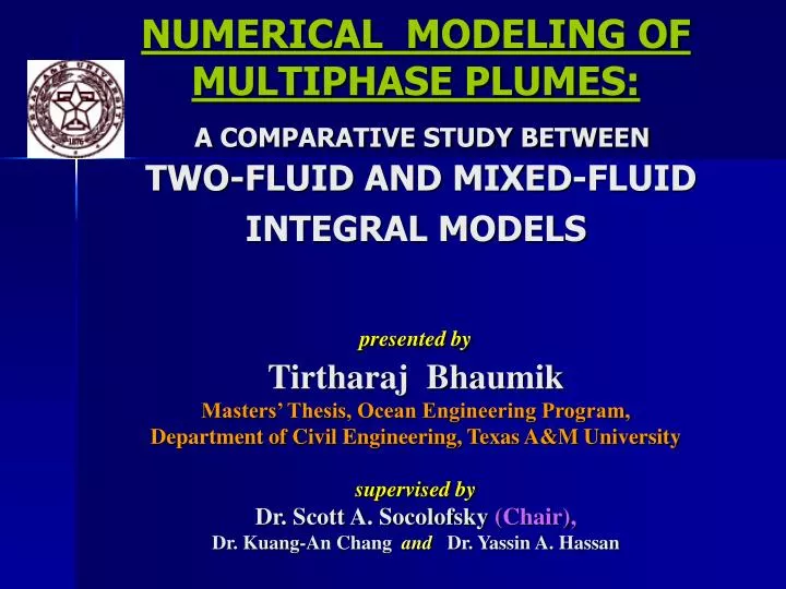
NUMERICAL MODELING OF MULTIPHASE PLUMES:A COMPARATIVE STUDY BETWEEN TWO-FLUID AND MIXED-FLUID INTEGRAL MODELSpresented byTirtharaj BhaumikMasters’ Thesis, Ocean Engineering Program, Department of Civil Engineering, Texas A&M Universitysupervised byDr. Scott A. Socolofsky (Chair),Dr. Kuang-An Chang and Dr. Yassin A. Hassan
OUTLINE • Multiphase Flow Terminologies • Two-fluid and Mixed-fluid Models • Governing Equations • Graphical User Interface • Initial Conditions • Model Verification with Experimental Data • Case Studies • Conclusion
MULTIPHASE FLOW TERMINOLOGY Multiphase flows are fluid flows involving the kinematics of more than one phase or constituent • Dispersed & Continuous Phases Dispersed Phase : Bubbles, Droplets, Powder Continuous Phase : Water, Air • Jets: Driving force – Momentum flux of dispersed phase • Plumes: Driving force – Buoyancy flux of dispersed phase
Two-fluid and Mixed-fluid models The Two-Fluid Model The Mixed-Fluid Model Dispersed phase Continuous phase Mixed Phase McDougall, 1978; Asaeda & Imberger, 1993 Socolofsky & Adams, 2001 WHICH MODEL YIELDS BETTER ESTIMATES ?
Multiphase Flow Applications • Bubble Breakwaters • Antifreeze measures in Harbors • Bubble curtains for Oil spill containment • Reservoir and Lake Destratification • Lake and Aquarium Aeration • CO2 Sequestration in Ocean • Blood flow modeling in bio-medical engineering • Two-phase flow modeling in chemical industries • Gas Stirring of molten metals in ladles, nuclear devices and chemical reactors
Ambient fluid (water) Outer plume hP H Inner Plume hT Air bubble Diffuser Source SCHEMATIC OF AN AIR-BUBBLE PLUME IN STRATIFIED AMBIENT
Ambient fluid (Water) Outer plume (Single phase) H hP Inner Plume (Mixed phase) hT Diffuser Source DOUBLE PLUME MODEL OF ASAEDA & IMBERGER (1993) (Mixed-fluid model)
Ambient fluid Outer plume (Continuous phase) hP H Inner Plume (Dispersed phase + Continuous phase) hT Bubble Core Diffuser Source DOUBLE PLUME MODEL OF SOCOLOFSKY & ADAMS (2001) (Two-fluid model)
MULTIPHASE PLUMES IN STRATIFIED ENVIRONMENT UN = us / (BN)¼ LIF Image of a Type 3 plume
Assumptions in Integral Models: 1. SELF – SIMILARITY ASSUMPTION 2. ENTRAINMENT HYPOTHESIS 3-D to 1-D Control Volume Top-Hat Distribution 3. DILUTE PLUME ASSUMPTION X: variable of interest ( u, C, ∆ρ)
Governing Differential equations: • 1. Conservation of Volume flux • 2. Conservation of Momentum flux • 3. Conservation of Buoyancy flux • 4. Conservation of Temperature flux • 5. Conservation of Concentration flux • 6. Conservation of Salinity flux • 7. Conservation of Mass flux of dispersed phase General Form of the model equations: …….. Coupled, non-linear ODEs Numerical Scheme : 4th order Runga-Kutta
Equation Balance: Flux variables (7 total): Primary variables (10 total): Closure Equations (3 additional): ……….. Sea-Water Equation of State ……….. Air/CO2 Equation of State ……….. Clift et. al (1978)
DIFFERENCE BETWEEN MIXED-FLUID AND TWO-FLUID MODELS Two-Fluid Model : Buoyant forces on twodistinct phases Mixed-Fluid Model : Buoyant force only on a singlemixed phase Control Volume (Axisymmetric)
DIFFERENCE BETWEEN MIXED-FLUID AND TWO-FLUID MODELS Conservation of Momentum flux …………… (Two-fluid model) ……………………………. (Mixed-fluid model)
DIFFERENCE BETWEEN MIXED-FLUID AND TWO-FLUID MODELS Conservation of Buoyancy flux …………… (Two-fluid model) ……………………………. (Mixed-fluid model) Mixture phase is transported at the velocity of the continuous phase ! Slip velocity of the dispersed phase not properly accounted for !
Ambient fluid SUBSEQUENT INNER PLUME INITIAL CONDITIONS Peel Height OUTER PLUME INITIAL CONDITIONS Trap Height hP H hT FIRST INNER PLUME INITIAL CONDITIONS Diffuser Source INITIAL CONDITIONS - (needed for each of the 7 flux variables in the model equations) - Of these, Q and J must be non-zero, otherwise there is a divide by zero error - However, u = 0 initially because a plume by definition has a zero initial velocity - Initial values of other flux variables can be obtained from the ambient properties • First Inner Plume • At release point (diffuser level) • Top of ZFE • Outer Plume • At the peeling locations • Subsequent Inner plumes • Just above the peeling locations
Zone of Established Flow Um Z0 = 10D Initial values of Um and b are calculated here b 5D Zone of Flow Establishment (ZFE) z = 0 Location of diffuser unit D 5D Location of virtual point source 1. VIRTUAL POINT SOURCE CONCEPT Cedarwall & Ditmars(1974), McDougall(1978) Single-phase plume equations are used up to the top of ZFE in order to predict non-zero values of b and Um at the start of computation (top of ZFE) First Inner plume Initial conditions: Fr = 1.7 0.025*H Fr = 0.8 2. DENSIMETRIC FROUDE NUMBER CONCEPT Wuest(1992) Multiphase plume formulation in terms of the Froude number can be used to predict non-zero values of b and Um at the start of computation (diffuser level) ZFE u = 0, b = 0
Ambient fluid SUBSEQUENT INNER PLUME INITIAL CONDITIONS Peel Height OUTER PLUME INITIAL CONDITIONS Trap Height hP H hT FIRST INNER PLUME INITIAL CONDITIONS Diffuser Source OUTER PLUME INITIAL CONDITIONS Extra Entrainment Fractional Peeling
EXPERIMENTAL SETUP 40 cm 40 cm 70 cm 10-bit 10-bit Q0= 0.5, 1.0, 1.5 l/min Bubble diameter = 3 mm 12-bit 532 nm 4 mm thick PIV/PTV 4 ms U is measured using PIV and Ub is measured using PTV
DETERMINATION OF MODEL PARAMETERS FROM EXPERIMENTAL DATA = 0.09 = 1.17 = 0.2 m/s
MODEL RUNS WITH INITIAL CONDITIONS OBTAINED EXPERIMENTALLY: Mixed-fluid model over-estimates momentum flux and continuous phase velocity
MODEL RUNS WITH MCDOUGALL’S (1978) INITIAL CONDITIONS Not very useful when the depth H is large
MODEL RUNS WITH WUEST’S (1992) INITIAL CONDITIONS No restrictions on water depth or diffuser diameter, hence more useful in general
MODEL RUNS WITH WUEST’S (1992) INITIAL CONDITIONS The Two-fluid model with Wuest’s initial conditions matches Froude number best
MODEL VERIFICATION WITH EXPERIMENTAL DATA IN A STRATIFIED AMBIENT Correlation of plume trap height to UN. Right-pointing triangles are data from Lemckert and Imberger (1993), circles are from Asaeda and Imberger (1993) and squares are from Socolofsky and Adams (2005). Open symbols are air-bubble experiments; closed symbols are glass bead experiments. Typical error bars are shown for one data point.
SENSITIVITY ANALYSIS FOR alpha Model results are sensitive to alpha, alpha = 0.09 gives best match
SENSITIVITY ANALYSIS FOR gamma Model results are insensitive to gamma, gamma = 1.2 is chosen
Case Studies • CASE 1:Lake Destratification • CASE 2:Lake Aeration • CASE 3:CO2 Sequestration in ocean
FIELD DATA FOR THE CASE STUDIES LAKE (Cases 1 and 2) OCEAN (Case 3) Source: Nepf (1995) Source: Teng et. al (1996) Density and Compressibility are calculated from the above data using EQUATION OF STATE
Case 1. Lake DestratificationMaintain water quality by artificial mixing,Prevent surface ice formation in winter Initial state Final state 50m N = f (z) N = 0 OBJECTIVE: Find optimal flow rate to achieve a well-mixed system
COMPARISON OF OPTIMAL FLOWRATE AS PREDICTED BY THE TWO MODELS db = 10 mm Q0 = 6.0 l/s (Mixed-Fluid model) Q0 = 15.0 l/s (Two-Fluid model)
Case 2. Lake AerationOxygenation below hypolimnion to prevent lake eutrophication in summer Hypolimnion 50m Air-bubble plume Diffuser port OBJECTIVE: Find optimal bubble diameter to dissolve all bubbles below hypolimnion
COMPARISON OF COMPUTED FLUX VARIABLES AS PREDICTED BY THE TWO MODELS db = 2 mm, Q0 = 6 l/s Mixed-fluid model predict higher values by about 30%
ESTIMATION OF DMPR BY THE TWO MODELS Smaller the bubbles, faster they dissolve Smaller the bubbles, lower is the slip velocity and hence less is the difference in the two model results
Case 3. CO2 SequestrationReduce greenhouse gas concentration in atmosphere by dumping carbon di-oxide in deep ocean in liquid form, Monitor pH change Atmosphere Ocean 800 m Multiphase plume of liquid CO2 droplets and water Phase change depth 350 m Pipeline Diffuser port OBJECTIVE: Find best combination of Q0 and db to dissolve all droplets below phase change depth
COMPARISON OF COMPUTED FLUX VARIABLES AS PREDICTED BY THE TWO MODELS db = 5 mm, Q0 = 1.1 l/s Mixed-fluid model predict higher values by about 40%
ESTIMATION OF DMPR BY THE TWO MODELS More the hydrate formation, lesser is the dissolution and hence higher is the DMPR Minimum Depth for hydrate formation: 450m in West Pacific, 820m in North Atlantic
CONCLUSIONS • The main difference between the mixed-fluid and the two-fluid models lies in the formulation of the conservation equation for momentum flux • In the existence of non-zero slip velocity and equal spreading ratios, the mixed-fluid model differs from the two-fluid model in the calculation of buoyant forces • The model results are sensitive to the entrainment coefficient (alpha) and the entrainment ratio (kappa), but insensitive to the value of the momentum amplification factor (gamma) • Wuest’s method of obtaining initial conditions for the first inner plume using the concept of bubble Froude number is the most reasonable and matches experimental data most closely • Typically, the mixed-fluid model is found to predict higher values of the peel height and the DMPR by about 30% as compared to the two-fluid model • Numerical simulations done using the two-fluid model gives more physically realistic, economic and more accurate designs


