Download
1 / 30
310 likes | 503 Views
The Art of Computer Performance Analysis. Raj Jain 1992 . Simulation. the distinction between simulation and emulation is fluid ns2 and other network simulators allow to attach real-world nodes; they can emulate “a network in between”.

E N D
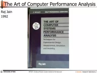
The Art of Computer Performance Analysis Raj Jain 1992
Simulation • the distinction between simulation and emulation is fluid • ns2 and other network simulators allow to attach real-world nodes; they can emulate “a network in between” • Where is simulation located in the system evaluation ecosystem? • analysis • simulation • emulation • evaluated prototype • evaluated deployed system no common term exists on these slides: “live testing” • the distinction between analysis and simulation is fluid • Queuing Theory, Markov Chains and Game Theory can blur the lines
Simulation • Pros • arbitrary level of detail • requires less theoretical understanding than analysis • allows simplifications compared to live systems • easier to explore parameter space than live systems • Cons • much slower than analytical approach • easy to wrongly avoid or oversimplify important real-world effects seen in live systems • bugs are harder to discover than in both, analytical approach and live systems
Simulation • When to choose simulation for a digital system? • too big to build • hardware not available • too expensive to build • essential performance parameters too complex to formulate analytically • too many variables to evaluate in a prototypical or deployed system • visual exploration of parameter space desirable
Simulation the set of all variables in a simulation that make it possible to repeat the simulation exactly at an arbitrary simulated time State State Variable one variable contributing to the state Event change in the system state
Simulation • Types of simulation
Simulation • Types of simulation
Simulation • Types of simulation
Simulation • Types of simulation Monte Carlo simulation often used for assessing static fairness, such as resource assignments (frequencies etc) • in Operating Systems and Networking,simulations have their origins in queuing theory • trace-driven and • discrete event simulation are prevalent
Simulation • Steady state is ... • ... in Monte Carlo simulation • the termination condition • the Monte Carlo simulation produces a meaningful results when (as soon as) steady state is reached • ... in discrete event simulation • reached when the influence of initialization values on state variables is no longer noticeable in simulation output • a simulation produces meaningful output after steady state is reached • ... in trace-driven simulation • like discrete event simulation
Simulation • Steady state in discrete event simulation • Generally steady state performance is interesting • Important exceptions exist, e.g. TCP slow start behaviour on a single link • when only steady state is interesting: transient removal • perform very long runs (wasting computing time) • ... or ... • truncation • initial (and final) data deletion • moving average of independent outputs • batch means
Simulation • How long to run a simulation? • Terminate conditions • in trace-driven simulation, event density drops, or trace ends • in discrete event simulation • termination event given by expert knowledge • variation in output value is narrow enough • variance of independent variable’s trajectory • variance of batch means
Simulation Common mistakes in simulation • invalid model: lacking realism • unverified model: bugs • inappropriate level of detail • no achievable goal • mysterious results • improper seed selection and too few runs with different seeds: representative situations are not covered • improperly handled initial conditions • inadequate user participation • inadequate time estimate too short: confidence of the results is too low
Simulation • Verification • modular design • anti-bugging (include self-checks) • structured walk-through (4 eyes principle) • deterministic model (known cases are simulated correctly) • trace (validate each step in simple cases) • graphical representation (validate visually) • continuity test (where applicable, small input changes result in small output changes) • degeneracy test (expected results reached with extreme variable settings) • consistency tests (more resources allow higher workload) • seed independence
Simulation • Validation is more difficult to achieve than for any other approach • Validation techniques • expert intuition • do results look as expected to an expert • real-system measurement • compare with practical results given by live testing • theoretical results • compare with analytical results for cases that can be modeled easily
Simulation The 3 rules of validation according to Jain Don’t trust the results of a simulation model until they have been validated by analytical modeling or measurements Don’t trust the results of an analytical model until they have been validated by a simulation model or measurements Don’t trust the results of a measurement until they have been validated by simulation or analytical modeling
Performance evaluation • Commonly used performance metrics • time • response time and reaction time • turnaround time: job start to completion • stretch factor: parallel vs sequential execution time • capacity • nominal: maximal achievable capacity under ideal workload • usable: maximal achievable with violating other conditions • throughput • efficiency • utilization • reliability • availability • objective quality • subjective metrics • subjective quality • mean opinion score • ranking of comparison pair
Performance evaluation • Workload selection • level-of-detail • representativeness • timeliness • loading level • test full load, worst case, typical case, procurement/target case • repeatability • impact of external components • don’t design a workload that is limited by external components
Performance evaluation Simplest way of evaluating data series: averaging mean variance standard deviation coefficient ofvariation
Performance evaluation Simplest way of evaluating data series: averaging • mode (for categorical variable like on/off or red/green/blue) • p-percentile • 1st quartile = 25-percentile • median = 2nd quartile = 50-percentile • 3rd quartile = 75-percentile
Common mistakes in performance eval no goals ignore input errors biased goals omitting assumptions and limitations unsystematic approach overlook important parameters inappropriate experiment design assuming no change in the future ignore significant factors unrepresentative workload(s) ignoring social aspects
Common mistakes in performance eval no analysis analyse without understanding the problem too complex analysis erroneous analysis wrong evaluation technique ignoring variability incorrect performance metric improper treatment of outliers improper presentation of results no sensitivity analysis
The Art of Data Presentation • Good charts • require minimal effort from the reader • maximize information • use words instead of symbols • label all axes clearly • minimize ink • no grid lines • more detail • use common practices • origin at (0,0) • cause along the x axis, effect on y axis • linear scales, increasing scales, equally divided scales
The Art of Data Presentation Checklist for line charts and bar charts (1/4):Line chart content • is the number of curves in the graph reasonably small? • can lines be distinguished from each other? • are the scales contiguous? • if the Y-axis presents a random quantity, are the confidence intervals shown? • is there a curve that can be removed without loosing information? • are the curves on a line chart labeled individually? • are all symbols explained? • if grid lines are shown, do they add information?
The Art of Data Presentation Checklist for line charts and bar charts (2/4):Bar chart content • are the bars labeled individually? • is the order of bars systematic? • does the area and width of bar charts represent (unequal) frequency and interval, respectively? • does the area and frequency of free space between bars convey information?
The Art of Data Presentation Checklist for line charts and bar charts (3/4):Labeling • are both coordinate axes shown and labeled? • are the axis labels self-explanatory and concise? • are the minimum and maximum values shown on the axes? • are measurement units indicated? • is the horizontal scale increasing left-to-right? • is the vertical scale increasing bottom-to-top? • is there a chart title? • is the chart title self-explanatory and concise?
The Art of Data Presentation Checklist for line charts and bar charts (4/4):General • is the figure referenced and used in the text at all? • does the chart convey your message? • would plotting different variables convey your message better? • do all graphs use the same scale? • does the whole chart provide new information to the reader?