Download
1 / 12
120 likes | 184 Views
This project focuses on integrating tides, self-attraction, and loading effects in ECCO estimates for improved circulation modeling. It explores the impact of SAL physics, long/short-period tides, and computational methods. The study aims to refine ocean mass calculations and circulation dynamics using efficient implementations and global convolution techniques.

E N D
Implementing tides and self-attraction and loading effects in ECCO estimates Rui M. Ponte Atmospheric and Environmental Research, Inc. Lexington, Massachusetts w/ Ayan Chaudhuri, Nadya Vinogradova, Katy Quinn, Sergey Vinogradov @AER and the ECCO group @MIT & JPL ECCO Meeting @ CalTech (Oct 31 - Nov 2, 2012)
What are we trying to do? • Allow for explicit interaction between tides and the general circulation in ECCO estimates • Develop an efficient implementation of self-attraction and loading (SAL) effects for tidal and non-tidal processes • Initial focus on improving circulation estimates (e.g., impacts on sea ice, dissipation, rectification effects) rather than modeling the tides • Re-examine long period tides and their static/dynamic nature in a full gcm setting • Assess impact of full treatment of SAL physics relative to commonly used scalar approximations
Tidal forcing • Tide potential acts essentially as atmospheric pressure (Ponte and Vinogradov 2007, JPO) and can be applied as such in the MITgcm • Traditional forcing method uses equilibrium tide potential for each relevant component (M2, S2, O1, K1, etc.) …preliminary tests with M2 based on ECCO version 4 setup underway • Possible to force with full potential, including all tide lines and their interactions at once …looking at adapting tidal codes developed by Thomas et al. (GRL, 2001) for the MITgcm
Long-period tides: an Mf solution Amplitude (dynamic term) • Largest dynamic response in the Arctic, some coastal areas and Southern Ocean • Large-scale Pacific, Atlantic pattern noticed in previous studies • Not strongly contaminated by circulation effects (including circulation effects)
Short-period tides: an M2 solution • Amplitude (m) and phase • Very first solution using version 4 setup • - Capturing most of the basic amplitude and phase patterns • - Missing some resonances (e.g., Mozambique channel, western Australian shelf) • - Generally weaker amplitudes (SAL effects not included yet) • -
Implications for time stepping • Difference in solutions with 5 minute (top) and 60 minute (bottom) time steps • - Long time step leads to much weaker amplitudes • - Raises important issues of time stepping schemes, implicit dissipation, and computational costs
Self-attraction and loading (SAL) • Self-gravitation and crustal loading processes, related to both ocean and other loads (land ice, hydrology, air mass), affect the ocean mass field and circulation • Effects commonly considered in tide modeling using an approximate constant factor modifying the tide forcing, but otherwise ignored in circulation estimates • At long time scales, iterative calculations can be done off line if the ocean response to loading can be treated as static (Tamisiea et al. 2010) • Full physics involves a global convolution at each time and between every grid point, which can incur extreme computational costs if done on a spatial grid (e.g. Stepanov and Hughes 2004) but can be done much faster using spherical harmonics (Schrama 2005) • Using scalar parameterizations can lead to substantial errors (Ray 1998, Stepanov and Hughes 2004) and static assumption is not universally valid
Basic method for SAL implementation SAL is a combination of three effects: direct gravitational attraction, seafloor loading and deformation, and changes in the Earth's gravity field due to the loading Overall SAL effect leads to a horizontal body force, implemented in the ocean model as a pressure loading, as with the tide potential Mass anomalies calculated from bottom pressure anomalies SAL is calculated using spherical harmonics to speed up computation, with spherical harmonic transformations performed using the efficient Driscoll and Healy (1994) sampling theorem Gridded bottom pressure → spherical harmonic bottom pressure → spherical harmonic SAL → gridded SAL Relatively low computational cost (6% CPU time increase in preliminary tests using version 4 setup)
Does scalar approximation work? • SAL is parameterized as 10% of bottom pressure (Stepanov and Hughes 2004) and results compared with the full SAL implementation
Discussion points • Ways to proceed in the short term • Assess other short-period tides, include parameterizations of barotropic/baroclinic tide interactions, apply SAL implementation, produce run with full tide treatment, analyze and understand impact of tides on the circulation,… • Test SAL codes fully, include effects of land loads (ice, hydrology, atmospheric pressure) • New physics brings higher costs and the need to decide what do we want to do about it • Study the problem to be able to parameterize it sufficiently well enough? Use optimization procedures to develop and fine tune parameterizations? • Do we want to estimate the tides as well as the circulation?