Download
1 / 41
410 likes | 577 Views
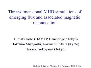
Three-dimensional MHD simulations of emerging flux and associated magnetic reconnection. Hiroaki Isobe (DAMTP, Cambridge / Tokyo) Takehiro Miyagoshi, Kazunari Shibata (Kyoto) Takaaki Yokoyama (Tokyo). 6th Solar-B Science Meeting, 8-11 November 2005, Kyoto. Outline.

E N D
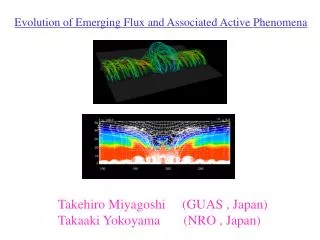
Three-dimensional MHD simulations of emerging flux and associated magnetic reconnection Hiroaki Isobe (DAMTP, Cambridge / Tokyo) Takehiro Miyagoshi, Kazunari Shibata (Kyoto) Takaaki Yokoyama (Tokyo) 6th Solar-B Science Meeting, 8-11 November 2005, Kyoto
Outline • Theories of magnetic reconnection and its difficulties • Huge magnetic Reynolds number • Scale gap • Key observations and its implication to theory • fractal nature of current sheet • plasmoid ejection • 3D MHD simulations of emerging flux and its reconnection with overlying coronal field • formation of filamentary structure • patchy reconnection • Observations by Solar-B
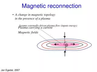
Theories of magnetic reconnection Sweet-Parker reconnection Reconnection rate: Parker 1957, Sweet 1958 Petschek reconnection Petschek 1964 • MHD simulations: if resistivity is localized, Petschek-like reconnection (i.e., with slow shocks) occurs. • Magnetosphere obs. and Lab experriments suggest that fast reconnection occurs when current sheet become as thin as ion Larmor radius or ion innertial length.
Fundamental problem in fast reconnection: huge scale gap • Laminar and steady reconnection with tiny diffusion region? Unlikely. • Mesoscale (MHD) structure? • Self-similar evolution in free space (Nitta P45)
Fractal nature of current sheets Hard X-ray emission (Ohki 1992) Fractal! Power spectrum of radio (610MHz) emission (Karlicky et al. 2005)
Fine spatial structure in reconnection events Small kernels in flare ribbons (Fletcher, Pollock & Potts 2004) aurora Supra-arcade downflows (McKenzie & Hudson 1999, Innes, McKenzie & Wang 2003, Asai et al. 2004 ) Surges/jets
Plasmoid (flux rope) ejection • Simultaneous acceleration of plasmoid and energy release • Slow rise and heating of plasmoid/flux rope prior to the hard X-ray burst
Laboratory experiment Reconnection rate is enhanced when current sheet (plasmoid) is ejected (Ono et al. 1997). Plasmoid-induced-reconnection (Shibata & Tanuma 2001)
Fractal current sheet with many islands? Tajima & Shibata 1997 Aschwanden 2002 • Consistent with the fractal nature of flare emission • Natural connection between MHD and micro scales
S-P type reconnection with enhanced resistivity? Turbulence? Vin/VA∝Rm-1/2 Vin/VA∝Rm-0.8 Statistical analysis of flares observed by Yohkoh/SXT Poster by Nagashima & Yokoyama, P43 Laboratory experiment (Ji et al. 1998)
MHD turbulence in reconnecting current sheet • Tearing instability (e.g., Furth et al. 1963, Shibata & Tanuma 2001...) • Secondary kink of tearing-made flux rope (Dahlburg, Antiochos & Zang 1992) • Kelvin-Helmholtz (Hirose et al. 2004) • Non-linear coupling of microinstabilities to macroscale (e.g., Shinohara et al. 2001) • Collision of reconnection jets (Watson & Craig 2003) • Reconnection-driven filamentation (Karpen, Antiochos & DeVore 1997) • Rayleigh-Taylor (indterchange) instability (Isobe et al. 2005)
Three-dimensional MHD simulation of emerging flux and reconnection with pre-existing coronal field Isobe, Miyagoshi, Shibata & Yokoyama 2005, Nature,434, 478
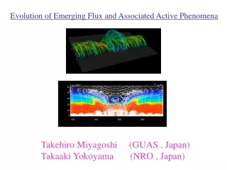
Observation of emerging flux region: Halpha • H alpha(104K) • Arch filament connecting the sunspots. • Why filament? (magnetic field must fill the space in the lowβ corona!) Matsumoto et al. 1993 Hα(Hida Obs.)
Observation of emerging flux region: EUV • EUV • Hot (T=106K) loops and cold (T=104K) loops exist alternatively • Intermittent coronal heating. • - Jets and flares... reconnection. TRACE EUV
2D MHD simulation(Yokoyama & Shibata 1995) Parker instability => emergence of loop in the corona => reconnection with pre-existing coronal field => jet
Simulation model • 3D extension of Yokoyama & Shibata (2005) • anomalous resistivity vd=J/ρ:ion-electron drift velocity • Upper convection zone - photosphere/chromosphere - corona • Horizontal magnetic sheet in the convection zon+uniform background field. • Grid: 800x400x620. Calculation was carried out using 160 processors of the Earth Simulator (about 8 hours for 50000 steps).
Result: overview Magnetic field lines Magnetic field lines + isosurface of |B| + temperature • Basically similar evolution to 2D simulation.
z y x Filamentary structure from the magnetic Rayleigh-Taylor instability • The top of the emerging flux becomes top-heavy=>unstable to the Rayleigh-Tyalor instability • Bending of magnetic field is stabilized=>Filamentary structure Color: mass density Hαimage of arch filaments Isosurface of mass density
Why top-heavy? Nonlinear evolution of Parker instability is approximately self-similar (Shibata et al. 1990). Field lines at different time density at middle simulation self-similar solution • The outermost part deviates from self-similar solution.
Why top-heavy? divvperp • The outermost field lines undergo: • Compression between coronal pressure above and magnetic pressure below. • Larger curvature radius => smaller gravity along B => less evacuation. divvpara
t=70 t=76 t=78 t=81 Evolution of the Rayleigh-Taylor instability Density at the y-z plane Fourier modes of Vz Linear growth rate • Small wavelength modes grow first (larger linear growth rate) • Larger scales from inverse cascade • Scale (width of filaments) may change with the presence of shear
Observational signature • Rayleigh-Taylor instability • Rising loops and (relatively) sinking loops exist alternatively. • Sinking loops are denser and probably colder • Spectroscopy in H-alpha and/or EUV • When the emerging loops become coronal temperature? • time scale of indivisual loop emergence 〜 1000 s • For EIS observations, time cadence is more important • Vortex excited by secondary Kelvin-Helmholtz instability • Tortional Alfven wave • Small scale twist in individual filaments • Chromospheric magnetic field measurement
z y x Formation of filamentary current sheets Mass density (contour) and current density (color) at the y-z cross section Mass density isosurface (gray) Current density distribution (color) • Deformation of magnetic field by the Rayleigh-Taylor instability =>current formation in the periphery of the dense filaments • Dissipation of these current sheets may result in intermittent heating, leading to the formation of the hot/cold loops system.
Reconnectin in the interchanging current sheet Anomalous resistivity B × ・ • Larger current density and smaller mass density in the rising part of the R-T instability • anomalous resistivity sets in locally • fast reconnection occurs in spatially intermittent way • Reconnection inflow enhance the nonlinear evolution of the R-T instability => nonlinear instability
Intermittent, patchy reconnection Isosurfaces of gas preasure + magnetic field line Many small plasmoids in the intialy laminar current sheet. • Isosurfaces of velocity. • Fast reconnection occurs in spatially intermittent way after the ejections of plasmoids. • Many narrow reconnection jets from initially laminar current sheet.
Conjecture • R-T instability can occur if there is density jump across the current sheet and effective acceleration (in suitable direction). • Effective acceleration is likely to exist in dynamically evolving system (like eruptive flares, CMEs, solarwind-magnetosphere) and in driven reconnections. • RT instability is ideal instability, hence no restriction from large Reynolds number. • Possible scenario may be... • Small scale turbulence grows by R-T instability (and couple with micro-scales) • tearing occurs in small scale • formation of large plasmoids (flux ropes) by coallescense => fast reconnection in global scale
Observation of reconnection signatures by Solar-B • Few spectroscopic detection of reconnection inflows/outflows (Innes et. al. 1997, Lin et al. 1995). =>EIS • Precise determination of the reconnection rate. • Slow shock? (Shiota et al. 2003) • Turbulent broadening Vturb ≈VAin hot temperature lines such as FeXXIV(10MK) if reconnection is fractal, i.e., many small reconnection.
Feasibility Temperature:T≈ 5-20MK. FeXXIV(192.08) is suitable?. Time scale: t≈ 10-100 (s). If turbulent-enhanced Sweet-Parker, the width of current sheet w is: w = MAL ≈ 10 - 1000 km. Assuming the (pre-flare) density of 109 cm-3, EM ≈ 1024-26 cm-5. For FeXXIV(192.028), several photons /s/pixel ... not easy but possible. (Thanks: Helen Mason)
3D structure of reconnection Same figure with isosurface of current density Magnetic field line + current density distribution • Petschek-like slow shocks
z y x Reconnection inflow/outflow in 3D Isosurface of |V| Velocity and current density on the x-z cross section Velocity on the y-z cross section in the outflow region. Contour is velocity perpendicular to the figure. Diverging Velocity on the y-z cross section in the outflow region. Converging • Outflow in diverging = more effective in plasma expelling. • => faster than 2D reconnection?
Comparison of the reconnection rate with 2D case Preliminaly. Reconnection rate measured by maximumηJ in the y-z cross section. • Locally, 3D reconnection is faster and more bursty than 2D reconnection. • The spatial average is comparable with 2D. • Rayleigh-Taylor does not occur in 2D... so the local condition near the reconnection point is not the same.
Summary • Filamentary structure spontaneously arises due to the magnetic Rayleigh-Taylor instability in the emerging flux. • Current sheets are formed in the periphery of arch filaments due to the R-T instability. Intermittent heating. • Magnetic reconnection becomes patchy, due to the interchanging of the current sheet. • Fine structure and dynamics in EFR filaments/loops (SOT/EIS/XRT) • Detection of reconnection inflows/outflows (EIS/XRT) • Turbulence in the current sheet (EIS) • EFR is suitable to target to catch the reconnection event (even in solar minimum).
Why top-heavy? Density in 2D simulations with coronal field without coronal field • Vertical distribution of density (color symbols) and Bx(solid) at the mid-point of the emerging flux. • Color indicates the Lagrangean trace of the fluid elements (i.e. same color indicates the same field lines.)
Divergence of the velocity components parallel and perpendicular to B divV divVperp • Top-heavy sheath locates at orange-magenta boundary. • Divergence of V (especially Vperp) changes the sign at this point. => convergence. divVpara
Deviation from self-similar solution (Shibata et a. 1990) simulation self-similar solution Density at the midpoint of the emerging flux. • The outermost part of emerging flux deviate from self-similar solution. • Compressed beteen coronal pressure and upward magnetic pressure from below (divVperp<0) • Outerfield lines have larger curvature radius and hence smaller effective gravity along B. (effect of divVpara)
t=10 t=80 Density@midpoint t=84 t=88 t=92 t=96 t=104 t=112
Helical flux rope • With the presence of the guide field (By), helical flux rope is formed. • (This calculation is still preliminary) Helical structure erupting after a prominence eruption (TRACE/EUV; Liu & Kurokawa 2004)
The Earth Simulator • A parallel vector computer system installed at the Earth Simulator Centre, in Yokohama, Japan. • Fastest computer in the world since 2002 until September 2004. ↓Tokyo Kyoto↓ ↑Yokohama
The Earth Simulator: hardware and software • 640 Processor Nodes (PNs) • One PN consists of 8 vector-type arithmetic processors (APs) and 16 GB shared memory.. • In total, 5120 APs and 10TB memory (distributed). • 40Tflops at peak, 35.86Tflops for Linpack Benchmark