Basic Microbiome Analysis with QIIME
Basic Microbiome Analysis with QIIME. Patricio Jeraldo and Bryan White. In this exercise you will. Calculate sample diversity ( a -diversity), and test if different sample types have different numbers of OTUs (species)


Basic Microbiome Analysis with QIIME
E N D
Presentation Transcript
Basic Microbiome Analysis with QIIME Patricio Jeraldo and Bryan White
In this exercise you will • Calculate sample diversity (a-diversity), and test if different sample types have different numbers of OTUs (species) • Calculate differences in microbial community structure (b-diversity): compare OTU composition and abundance between samples and sample types • Compute statistical support for observed differences between sample types • Plot taxonomy composition across samples • Test for potential microbial markers
Tools and data • We will use QIIME, installed in biocluster • Data set is also located in biocluster • QIIME returns some results as interactive web pages: we will run all commands in biocluster first, then move the results to the desktop and view the results there.
Exercise: Interstitial cystitis • Cohort: 15 women (8 with IC, 7 controls) • 16S sequencing of stool samples • Hypothesis: IC induces significant changes in gut microbiota • Other questions: is it a change in the community? Is a specific bacteria responsible for the change?
Step 0: connect to biocluster • Open the program PuTTY and connect to the cluster with your credentials
Step 1: create a directory • To create a directory to store a copy of the data set, type: • And change directory to the newly created one: mkdirmicrobiome cd microbiome
Step 2: copy the dataset • The zip file with the data set is in a different directory. Let’s copy it to our own: Let’s make sure it’s there: You should see the following: cp /home/groups/chian_tornado/workshop/*.zip . ls ICF.microbiome.zip
Step 3: unpack the dataset • Let’s unpack the dataset: And list the files we have so far: We see 4 files were extracted from the zip file. Let’s go over them… unzip ICF.microbiome.zip ls ICF.biomICF.mapping.txtICF.microbiome.zipICF.treeparams.txt
Step 3a: BIOM file • OTU observation file. It is a matrix of observed OTUs (species) for each sample, annotated with their taxonomy. • Created using our own TORNADO pipeline for 16S reads: quality check, chimera check, align, assign taxonomy and cluster to 97% similarity to find OTUs (pipeline can take hours to days!).
Step 3b: mapping file • File with metadata associated with samples. Check its contents: cat ICF.mapping.txt #SampleIDBarcode DxSubjectID Description ICF-1 GGATCGCAGATC Control 1 IC_fecal1 ICF-2 GCTGATGAGCTG Control 2 IC_fecal2 ICF-3 AGCTGTTGTTTG Control 3 IC_fecal3 ICF-4 GGATGGTGTTGC IC 4 IC_fecal4 … …
Step 3b: mapping file • In our case, the most important column is marked as Dx • In your own analysis, you must supply the metadata! #SampleID Barcode DxSubjectID Description ICF-1 GGATCGCAGATC Control 1 IC_fecal1 ICF-2 GCTGATGAGCTG Control 2 IC_fecal2 ICF-3 AGCTGTTGTTTG Control 3 IC_fecal3 ICF-4 GGATGGTGTTGC IC 4 IC_fecal4 …
Step 3c: tree file • Newick-formatted phylogenetic tree file • Contains phylogenetic relationships between the different OTUs (species) found in the samples • Another output of the 16S pipelines • Required for some comparison metrics
Step 3d: params file • File with parameters for QIIME • Needed only when changing default analyses • Let’s see its contents: • It specifies the comparison metrics to use in analyses we will be doing. cat params.txt beta_diversity:metricsbray_curtis,unweighted_unifrac,weighted_unifrac alpha_diversity:metrics chao1,goods_coverage,observed_species,shannon,simpson,PD_whole_tree
Step 4: results directory • Last step before diving into the analysis, let’s create a results directory to store our data mkdir results
Step 5: interactive cluster session • Let’s create an interactive session in the cluster: each of us will have our own processor to perform the analyses • Now, change again to our microbiome directory qsub -I cd microbiome
Step 6: load the QIIME module • Let’s load the qiime module • This makes the QIIME scripts available to us, as well as other software QIIME needs (python, R, etc…) module add qiime
Step 7: library stats • Let’s do a quick check on our BIOM file • Note the minimum number of seqsin the library. We will use this number to better compare the different samples… per_library_stats.py –I ICF.biom Num samples: 15 Numotus: 260 Num observations (sequences): 399985.0 Table density (fraction of non-zero values): 0.6082 Seqs/sample summary: Min: 10267.0 Max: 48123.0 …
Step 8: a-diversity • Let’s measure the diversity of the samples. We will use the number from the previous slide so that, for comparison purposes, all samples will have the same number of sequences… • The results will be stored in the results/alpha_diversity directory as interactive web pages and other files. alpha_rarefaction.py –I ICF.biom –t ICF.tree –m ICF.mapping.txt –o results/alpha_diversity –p params.txt –e 10267 This calculation will take from 5 to 7 minutes to complete
Step 9: b-diversity • Now let’s compare all samples using their composition, also specifying that we’re interested in the Dx column. • The results will be stored in the results/beta_diversity directory as interactive web pages and other files. We will be using some of those files as input for further analysis. beta_diversity_through_plots.py –I ICF.biom –t ICF.tree –m ICF.mapping.txt –o results/beta_diversity –p params.txt –e 10267 –c Dx This calculation will take about 5 minutes to complete
Step 9: taxonomy • Let’s create a graphical summary of the taxonomical composition of the samples • Also, let’s do the same but merging the control and the IC samples (using the Dx column) • The results will be stored in the results/taxonomy directory as interactive web pages and other files. summarize_taxa_through_plots.py –I ICF.biom –m ICF.mapping.txt –o results/taxonomy summarize_taxa_through_plots.py –I ICF.biom –m ICF.mapping.txt –o results/taxonomy_Dx–c Dx
Step 10: ANOVA tests • Let’s see if there are OTUs (species) that explains the differences between the sample categories. We will do that using an ANOVA test… • The resulting file, ANOVA.txt, sorts the OTUs in the data according to how likely they are driving the differences between samples. The file includes probabilities (uncorrected and corrected), as well as abundance information and lineage of the OTU. otu_category_significance.py –iICF.biom –m ICF.mapping.txt –o results/ANOVA.txt –s ANOVA –c Dx
Statistical tests • If the control and IC samples cluster together, the following tests will measure the significance of such clustering based on the metrics that we just calculated…
Step 11: a-diversity significance • Let’s see if control and IC cases differ significantly in number of observed OTUs, using our previous a-diversity calculation… • Let’s look at the output: • It seems that the categories are very different… we will confirm this later when looking at diversity plots. compare_alpha_diversity.py –i results/alpha_diversity/alpha_div_collated/observed_species.txt –c Dx –o results/species_significance.txt –d 10260 cat results/species_significance.txt Comparisontvalpval Control,IC 3.65454556682 0.002
Step 12: b-diversity significance • Let’s compare the categories again, this time using the output from the b-diversity calculations. In particular we will use the UniFrac matrix… Let’s perform an ANOSIM test. • Now let’s take a look at those results… • Although the p-value is significant, the R statistic says that the clustering is only moderately strong. compare_categories.py –-method anosim –i results/beta_diversity/unweighted_unifrac_dm.txt –m ICF.mapping.txt –c Dx –o results/anosim –n 9999 cat results/anosim/anosim_results.txt Method name R statistic p-value Number of permutations ANOSIM 0.4694 0.0008 9999
Packing the results • Now let’s pack the results directory • The zip file now can be transferred to your computer. Do so, and then unpack it. We will explore the results through the interactive web pages QIIME created for us. zip –r results.zip results
Results: a-diversity • Inside the results directory, navigate to alpha_diversity -> alpha_rarefaction_plots and open rarefaction_plots.html • Select observed_species as metric, and Dx as category. A graph will be displayed.
Results: b-diversity • Now let’s look at the ordination plots for the samples. Go to beta_diversity -> unweighted_unifrac_2d_discrete and open the HTML file • This will open a 2d PCA plot, based on unweightedUniFrac distances, colored by sample type (Dx, Control)
Results: b-diversity Hover on the data points to obtain information about that sample…
Control and IC samples segregate, but only moderately. This is in agreement with the ANOSIM results (R=0.4694 , p = 0.0008).
Results: taxonomy • Let’s examine the taxonomy results. In the results directory, go to taxonomy -> taxa_summary_plots and open area_charts.html
This is the taxonomy at phylum level, for all samples. Hover over each color to find out about each color (colors may differ from this plot). • These look like otherwise normal stool samples, with Firmicutes and Bacteroides dominating. Note the Fusobacteria in sample 2, a control!
Things get more complex as we go down the taxonomy hierarchy. This is the plot at genus level, typical of stool samples. There seems to be no obvious pattern, the usual case unless there’s something very wrong, or a known pathogen. Hover over each color to see its taxonomy information.
Let’s see if there is something hidden in the taxonomy. In the results directory, open the ANOVA.txt file. OTU probBonferroni_correctedFDR_correctedControl_meanIC_mean Consensus Lineage 111 0.000113443547213 0.0250710239341 0.0250710239341 0.00310594468968 0.00022022007532 k__Bacteria; p__Bacteroidetes; c__Bacteroidia; o__Bacteroidales; f__Porphyromonadaceae; g__Odoribacter; s__unclassified 22 0.00128127076471 0.283160839001 0.1415804195 0.0155471912415 0.00128661622402 k__Bacteria; p__Firmicutes; c__Clostridia; o__Clostridiales; f__Lachnospiraceae; g__unclassified; s__unclassified 89 0.00148832607004 0.328920061478 0.109640020493 0.00408471212469 0.000983251999578 k__Bacteria; p__Firmicutes; c__Clostridia; o__Clostridiales; f__Lachnospiraceae; g__Clostridium; s__unclassified 154 0.0025315674133 0.559476398339 0.139869099585 7.38470627331e-06 0.00183392914333 k__Bacteria; p__Tenericutes; c__Erysipelotrichi; o__Erysipelotrichales; f__Erysipelotrichaceae; g__Clostridium; s__Clostridium_ramosum Odoribacter has 0.3% abundance in controls, 0.02% in IC…
Indeed, it seems to be a good marker despite its low relative abundance. Its absence seems correlated with IC (samples 4,7,8,9,10,12,14,15).
Analysis conclusions • Microbial composition and structure significantly different in stool between IC patients and controls: • IC stool microbiotasignificantly less diverse • Overall IC microbiota different (it clusters away from controls) • Potential marker found • Lack of Odoribacter associated with IC
Exercise conclusions • Basic microbiome analysis: • Calculate various diversity metrics for samples • Calculate statistical support for differences found between samples types • Plot taxonomy composition of samples • Basic tests for potential microbial markers