Download
1 / 32
320 likes | 519 Views
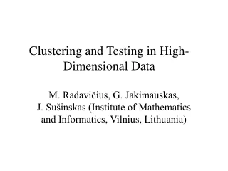
Clustering and Indexing in High-dimensional spaces. Outline. CLIQUE GDR and LDR. CLIQUE (Clustering In QUEst). Agrawal, Gehrke, Gunopulos, Raghavan (SIGMOD’98). Automatically identifying subspaces of a high dimensional data space that allow better clustering than original space

E N D
Outline • CLIQUE • GDR and LDR
CLIQUE (Clustering In QUEst) • Agrawal, Gehrke, Gunopulos, Raghavan (SIGMOD’98). • Automatically identifying subspaces of a high dimensional data space that allow better clustering than original space • CLIQUE can be considered as both density-based and grid-based • It partitions each dimension into the same number of equal length intervals • It partitions an m-dimensional data space into non-overlapping rectangular units • A unit is dense if the fraction of total data points contained in the unit exceeds the input model parameter • A cluster is a maximal set of connected dense units within a subspace
CLIQUE: The Major Steps • Partition the data space and find the number of points that lie inside each cell of the partition. • Identify the subspaces that contain clusters using the Apriori principle • Identify clusters: • Determine dense units in all subspaces of interests • Determine connected dense units in all subspaces of interests. • Generate minimal description for the clusters • Determine maximal regions that cover a cluster of connected dense units for each cluster • Determination of minimal cover for each cluster
Vacation(week) 7 6 5 4 3 2 1 age 0 20 30 40 50 60 Vacation 30 50 Salary age Salary (10,000) 7 6 5 4 3 2 1 age 0 20 30 40 50 60 = 3
Strength and Weakness of CLIQUE • Strength • It automatically finds subspaces of thehighest dimensionality such that high density clusters exist in those subspaces • It is insensitive to the order of records in input and does not presume some canonical data distribution • It scales linearly with the size of input and has good scalability as the number of dimensions in the data increases • Weakness • The accuracy of the clustering result may be degraded at the expense of simplicity of the method
High Dimensional Indexing Techniques • Index trees (e.g., X-tree, TV-tree, SS-tree, SR-tree, M-tree, Hybrid Tree) • Sequential scan better at high dim. (Dimensionality Curse) • Dimensionality reduction (e.g., Principal Component Analysis (PCA)), then build index on reduced space
Global Dimensionality Reduction (GDR) First Principal Component (PC) First PC • works well only when data is globally correlated • otherwise too many false positives result in high query cost • solution: find local correlations instead of global correlation
Cluster1 First PC of Cluster1 Cluster2 First PC of Cluster2 Local DimensionalityReduction (LDR) GDR LDR First PC
Correlated Cluster Mean of all points in cluster Centroid of cluster (projection of mean on eliminated dim) First PC (retained dim.) Second PC (eliminated dim.) A set of locally correlated points = <PCs, subspace dim, centroid, points>
Reconstruction Distance Centroid of cluster Projection of Q on eliminated dim Point Q First PC (retained dim) Reconstruction Distance(Q,S) Second PC (eliminated dim)
Reconstruction Distance Bound Centroid £ MaxReconDist First PC (retained dim) £ MaxReconDist Second PC (eliminated dim) ReconDist(P, S) £ MaxReconDist, " P in S
Other constraints • Dimensionality bound: A cluster must not retain any more dimensions necessary and subspace dimensionality £ MaxDim • Size bound: number of points in the cluster ³ MinSize
Clustering Algorithm Step 1: Construct Spatial Clusters • Choose a set of well-scattered points as centroids (piercing set) from random sample • Group each point P in the dataset with its closest centroid C if the Dist(P,C) £ e
Clustering Algorithm Step 2: Choose PCs for each cluster • Compute PCs
Clustering AlgorithmStep 3: Compute Subspace Dimensionality • Assign each point to cluster that needs min dim. to accommodate it • Subspace dim. for each cluster is the min # dims to retain to keep most points
Clustering Algorithm Step 4: Recluster points • Assign each point P to the cluster S such that ReconDist(P,S) £ MaxReconDist • If multiple such clusters, assign to first cluster (overcomes “splitting” problem) Empty clusters
Clustering algorithmStep 5: Map points • Eliminate small clusters • Map each point to subspace (also store reconstruction dist.) Map
Clustering algorithmStep 6: Iterate • Iterate for more clusters as long as new clusters are being found among outliers • Overall Complexity: 3 passes, O(ND2K)
Experiments (Part 1) • Precision Experiments: • Compare information loss in GDR and LDR for same reduced dimensionality • Precision = |Orig. Space Result|/|Reduced Space Result| (for range queries) • Note: precision measures efficiency, not answer quality
Datasets • Synthetic dataset: • 64-d data, 100,000 points, generates clusters in different subspaces (cluster sizes and subspace dimensionalities follow Zipf distribution), contains noise • Real dataset: • 64-d data (8X8 color histograms extracted from 70,000 images in Corel collection), available at http://kdd.ics.uci.edu/databases/CorelFeatures
Index structure Root containing pointers to root of each cluster index (also stores PCs and subspace dim.) Set of outliers (no index: sequential scan) Index on Cluster 1 Index on Cluster K Properties: (1) disk based (2) height £ 1 + height(original space index) (3) almost balanced
For each cluster S, multidimensional index on (d+1)-dimensional space instead of d-dimensional space: NewImage(P,S)[j] = projection of P along jth PCfor 1 £ j £ d = ReconDist(P,S) for j= d+1 Better estimate: D(NewImage(P,S), NewImage(Q,S)) ³ D(Image(P,S), Image(Q,S)) Correctness: Lower Bounding Lemma D(NewImage(P,S), NewImage(Q,S)) £ D(P,Q) Cluster Indices
Outlier Index • Retain all dimensions • May build an index, else use sequential scan (we use sequential scan for our experiments)
Query Support • Correctness: • Query result same as original space index • Point query, Range Query, k-NN query • similar to algorithms in multidimensional index structures • see paper for details • Dynamic insertions and deletions • see paper for details
Experiments (Part 2) • Cost Experiments: • Compare linear scan, Original Space Index(OSI), GDR and LDR in terms of I/O and CPU costs. We used hybridtree index structure for OSI, GDR and LDR. • Cost Formulae: • Linear Scan: I/O cost (#rand accesses)=file_size/10, CPU cost • OSI:I/O cost=num index nodes visited, CPU cost • GDR:I/O cost=index cost+post processing cost (to eliminate false positives), CPU cost • LDR:I/O cost=index cost+post processing cost+outlier_file_size/10, CPU cost
Conclusion • LDR is a powerful dimensionality reduction technique for high dimensional data • reduces dimensionality with lower loss in distance information compared to GDR • achieves significantly lower query cost compared to linear scan, original space index and GDR • LDR has applications beyond high dimensional indexing