Download
1 / 34
340 likes | 358 Views
This presentation highlights the findings of a meta-analysis of two SP data sets from Gauteng. It focuses on choice model design, discrete choice model results, and the implications for understanding travel preferences. The analysis evaluates the value of behavioral travel time savings, traveler heterogeneity, and the suitability of conjoint models. The results provide valuable insights for transportation planning in the region.

E N D
A Meta-Analysis of Two Gauteng SP Data Sets Presentation to Southern African Transport Conference Gary Hayes Prof. Christo Venter 11th July 2017
Presentation Overview • Choice Model Design Process • SP Experiments & Discrete Choice Models (DCM) • Background to Tshwane and Ekurhuleni SP Data Sets • Discrete Choice Model Results • What does this tell us?
1. The Choice Model Design Process • What user choices are to be simulated? • Implications for model structure; • Utility function definition & attributes (focus groups); • Market segments & sample sizes. 1 Design of choice model Design & Execution of SP / RP Experiment 2 • Capture device & type of survey (e.g. CAPI intercept) • Attribute levels, orthogonal designs, fractional factorial designs (i.e. no. of choice sets & blocks); • Pilot surveys, revisions & main surveys. 3 Estimation of Discrete Choice Model (DCM) • Appropriate software (incl. freeware e.g. Biogeme, R); • Overall model and individual attribute statistical significance; • Interpretation & application of outputs.
2. Stated Preference Experiments • Used to determine user preferences for products / services using choice models; • Require respondents to make a CHOICE between alternatives; • Respondents make their choice based on trip time, cost and transfer trade-offs. Example of a choice set (labelled) RP SP
Integration of mode choice model and SP survey design (SP Outputs = Mode Choice model inputs). 2. SP Surveys - Key Requirements Inclusion of RP and pivoting SP off RP. Questionnaire completion time and type of survey. Use of CAPI must be standard. Pilot survey essential. Mode Choice Model Design and SP Survey Design SP Survey fieldwork training, management and constant monitoring. • Fractional factorial & orthogonal choice set designs.
2. Discrete Choice Models (DCM’s) Choice process of individual n: • DCM’s use utility theory to explain user preferences • Random utility maximisation is fundamental to DCM’s • Several types, e.g. multinomial logit (MNL), nested logit and mixed logit (ML) models.
2. Definition of Trip Utility Standard Form of Utility: Linear in Parameters form of weighted attributes Weighted Sum of Observable Attributes Unobservable ‘Random’ Component Utility of Alternative + = Utility of Alternative iwith n attributes= μi= Σ βinX+εi n n=1 Systematic / Deterministic component common to all individuals. Also known as Representative Utility Notes Stochastic Component unique to individuals + • As we cannot ‘read the mind’ of the individual and exactly predict their choice, • we can only explain choice up to a probability of selection; • VTTS is the marginal rate of travel time divided by marginal rate of travel cost • i.e. Behavioural VTTS = ratio of travel time and cost β values 7
3. The Three SP Data Sets in Gauteng • SP Survey for Proposed BRT Mode: • Sample size: 400 • Current Modes: Minibus taxi; rail; bus; car • Alternative mode: BRT • Rated responses (5-point Likert); • Conjoint analysis for MNL application Tshwane (2012) • SP Survey for Proposed BRT Mode: • Sample size: 400 • Current Modes: Minibus taxi; rail; car • Alternative mode: BRT • Rated responses (5-point Likert); • Conjoint analysis for MNL application Ekurhuleni (2013) • SP/RP Survey for BRT Mode Evaluation: • Sample size: 1,200 • Current Modes: Minibus taxi; rail; car; Gautrain; bus • CAPI survey with alternative attributes pivoted off current mode values • Alternative mode: BRT • Mixed logit application Johannesburg (2014)
3. Objectives of SP Meta-Analysis Four main objectives of the investigation were: Estimate Value of Behavioural Travel Time Savings (VTTS) Evaluate Extent of Traveller Heterogeneity Assess Suitability of Conjoint Models Consolidate Tshwane and Ekurhuleni SP Data Sets
4. Conversion Assumption: Likert to Choice Responses The key assumptions were that: If a respondent prefers or strongly prefers their current mode, the discrete choice is 0; If they prefer or strongly prefer the alternative (BRT) mode, then the discrete choice is 1; If the response was neutral it was removed for the data set.
4. City of Tshwane CM and MNL Results: All Income Groups Bus mode excluded from public modes Conjoint Model Original VTTS all modes all income groups: R5.31/hr Note: Behavioural VTTS is not the same as social or equity VTTS used in economic analyses. MNL
4. Ekurhuleni CM and MNL Results (All Incomes) Conjoint Model Original VTTS: Rail: R8.89/hr Taxi: R14.72/hr Car: R83.36/hr MNL
4. Tshwane and Ekurhuleni Consolidated MNL & ML Results (All incomes): Mode VTTS Heterogeneity MNL Mixed Logit
4. Tshwane + Ekurhuleni: Car 95% VTTS Confidence Intervals Mean VTTS R29.65/hr Mean VTTS R25.18/hr
4. Jo’burg MNL & ML VTTS 95% Confidence Intervals by Mode & Income
4. What if We get the Choice Model and VTTS Wrong? Ex post B/C evaluation of Rea Vaya Ph 1A TTS Share of total benefits = 37% VTTS used = R56/hr BCR = 1.19 At VTTS of R34/hr (-40%), estim. pass = -5% BCR=1.0 19 19 10 July 2017 10 July 2017 Source: EMBARQ: Social, Environmental and Economic Impacts of BRT systems: Bus Rapid Transit Case Studies from Around the World, 2014
5. Conclusions • We still don’t have sufficient insight into travel behaviour and willingness to pay – there are large gaps; • VTTS is lower than estimated in the past; • We must be aware of pitfalls of ‘one size fits all’ transport systems and operations; • In some cases we may have made the wrong feasibility & infrastructure design and operations decisions; • We have to invest in behavioural research when making investment decisions worth R(billions); • We might make the same decisions, but be more aware of the downside risks, and mitigation strategies. We normally get the forecasts wrong. When we get it right it’s for the wrong reasons
Transit Assignment: Why Logit-Based Methods are Required for South African Transit Networks Presentation to Southern African Transport Conference Gary Hayes Prof. Christo Venter 11th July 2017
Presentation Overview • Where does transit assignment fit in? • What is transit assignment so difficult to calibrate? • Optimal Strategy and the Common Line Problem • Logit-Based Transit Assignment • What does this tell us?
1. Mode Choice – Assignment Process Note:Behavioural attributes and weightings must be used in mode choice and assignment models.
2. Why is Transit Assignment Difficult to Calibrate? Common line problem Transit Assignment Decision Rules Limited Time Period Models (e.g. 1 hour) Transit Operations Coding: Routes, Headways, Speeds, Fares, Stops. Transit Assignment Limitations Effect of technology on choice? Large traffic zones don’t help Capacity Constraints not Modelled Static, Average Headway based Models Behavioural data: time & cost weightings
2. Why is Transit Assignment to Difficult to Calibrate? Transit assignment calibration is notoriously difficult - goodness of fit criteria are hard to achieve; Rail = Easiest Taxi = Hardest Bus = Harder
3. Optimal Strategy & The Common Line Problem • A strategy is a set of attractive lines at each boarding decision point encountered by the traveller • The optimal strategy is the minimum generalized cost path; • Common lines can distort the assignment: will all the trips on Route 1 (with end station destination) interchange at Station 2 and use Route 2 if there are marginal travel time savings on Route 2?
3. Optimal Strategy & The Common Line Problem i Total Person trips i to j by taxi from MNL = 100 per hour • A Optimal taxi strategy is Taxi Line 3 Transit assignment result: Taxi Line 3 Taxi Line 1 Taxi Line 2 • Comments: • Arrangement of centroid connectors is critical; • Unrealistic transit assignment result, trips should be spread between three lines; • Difficult to calibrate model link volumes based on transit assignment result; • Using trip matrix estimation approach to estimate base matrices will give incorrect trip ends and incorrect final matrix.
4. Variant Transit Assignment (Florian & Constantin) • P(line i) is the likelihood of a traveller choosing line i; • Θx is the unique scale factor for zone x (value between 0 and 1) that limits the number of competing strategies included in the solution. A value of 0 includes all strategies & value of 1 includes only the cheapest strategy; • n is the number of lines between O-D included in the strategy; • (Util i) is the trip utility of line i between O-D.
4. Zenith Transit Assignment (Brands, de Romph, Veitch) • Features: • Centroid connectors automatically generated within centroid radius; • Type of transit stop / station can be defined, e.g. park and ride; • Minimum number of stops within radius can be defined (i.e. define more stops or increase radius); • Transit systems that must be reached. • P(line i) is the likelihood of a traveller choosing line i; • Fi is the frequency of line i; • Θx is the zonal service choice parameter (i.e. scale factor) for zone x; • n is the number of lines between O-D; • (Cost i) is the total trip generalised cost of line i between O-D.
4. Zenith Transit Assignment (Brands, de Romph, Veitch) Taxi line demand with variation in Line 3 frequency and θ = 0.2.
Conclusions • Considered mode choice / assignment models are necessary; • Alternative approaches to standard transit assignment should be investigated; • DCM behavioural data must be used in mode choice and traffic & transit assignment models; • Variant transit assignment approach is relatively simple to implement and automate for zonal scale factor estimation.