Download
1 / 30
300 likes | 581 Views
Analysis Overheads. 2. Transformations. Some effect size types are not analyzed in their

E N D
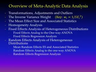
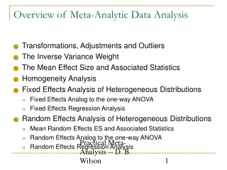
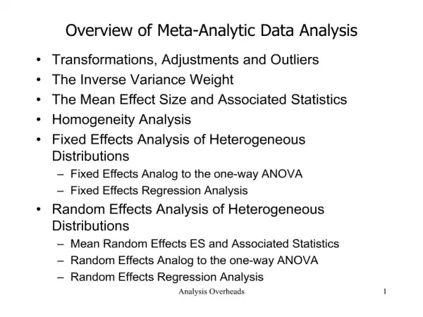
1. Analysis Overheads 1 Overview of Meta-Analytic Data Analysis Transformations, Adjustments and Outliers
The Inverse Variance Weight
The Mean Effect Size and Associated Statistics
Homogeneity Analysis
Fixed Effects Analysis of Heterogeneous Distributions
Fixed Effects Analog to the one-way ANOVA
Fixed Effects Regression Analysis
Random Effects Analysis of Heterogeneous Distributions
Mean Random Effects ES and Associated Statistics
Random Effects Analog to the one-way ANOVA
Random Effects Regression Analysis
2. Analysis Overheads 2
3. Analysis Overheads 3 Transformations (continued) Correlation has a problematic standard error formula.
Recall that the standard error is needed for the inverse variance weight.
Solution: Fisher�s Zr transformation.
Finally results can be converted back into �r� with the inverse Zr transformation (see Chapter 3).
4. Analysis Overheads 4 Transformations (continued) Analyses performed on the Fisher�s Zr transformed correlations.
Finally results can be converted back into �r� with the inverse Zr transformation.
5. Analysis Overheads 5 Transformations (continued) Odds-Ratio is asymmetric and has a complex standard error formula.
Negative relationships indicated by values between 0 and 1.
Positive relationships indicated by values between 1 and infinity.
Solution: Natural log of the Odds-Ratio.
Negative relationship < 0.
No relationship = 0.
Positive relationship > 0.
Finally results can be converted back into Odds-Ratios by the inverse natural log function.
6. Analysis Overheads 6 Transformations (continued) Analyses performed on the natural log of the Odds- Ratio:
Finally results converted back via inverse natural log function:
7. Analysis Overheads 7 Adjustments Hunter and Schmidt Artifact Adjustments
measurement unreliability (need reliability coefficient)
range restriction (need unrestricted standard deviation)
artificial dichotomization (correlation effect sizes only)
assumes a normal underlying distribution
Outliers
extreme effect sizes may have disproportionate influence on analysis
either remove them from the analysis or adjust them to a less extreme value
indicate what you have done in any written report
8. Analysis Overheads 8 Overview of Transformations, Adjustments,and Outliers Standard transformations
sample sample size bias correction for the standardized mean difference effect size
Fisher�s Z to r transformation for correlation coefficients
Natural log transformation for odds-ratios
Hunter and Schmidt Adjustments
perform if interested in what would have occurred under �ideal� research conditions
Outliers
any extreme effect sizes have been appropriately handled
9. Analysis Overheads 9 Independent Set of Effect Sizes Must be dealing with an independent set of effect sizes before proceeding with the analysis.
One ES per study OR
One ES per subsample within a study
10. Analysis Overheads 10 The Inverse Variance Weight Studies generally vary in size.
An ES based on 100 subjects is assumed to be a more �precise� estimate of the population ES than is an ES based on 10 subjects.
Therefore, larger studies should carry more �weight� in our analyses than smaller studies.
Simple approach: weight each ES by its sample size.
Better approach: weight by the inverse variance.
11. Analysis Overheads 11 What is the Inverse Variance Weight? The standard error (SE) is a direct index of ES precision.
SE is used to create confidence intervals.
The smaller the SE, the more precise the ES.
Hedges� showed that the optimal weights for meta-analysis are:
12. Analysis Overheads 12 Inverse Variance Weight for theThree Major League Effect Sizes Standardized Mean Difference:
13. Analysis Overheads 13 Inverse Variance Weight for theThree Major League Effect Sizes Logged Odds-Ratio:
14. Analysis Overheads 14 Ready to Analyze We have an independent set of effect sizes (ES) that have been transformed and/or adjusted, if needed.
For each effect size we have an inverse variance weight (w).
15. Analysis Overheads 15 The Weighted Mean Effect Size Start with the effect size (ES) and inverse variance weight (w) for 10 studies.
16. Analysis Overheads 16 The Weighted Mean Effect Size Start with the effect size (ES) and inverse variance weight (w) for 10 studies.
Next, multiply w by ES.
17. Analysis Overheads 17 The Weighted Mean Effect Size Start with the effect size (ES) and inverse variance weight (w) for 10 studies.
Next, multiply w by ES.
Repeat for all effect sizes.
18. Analysis Overheads 18 The Weighted Mean Effect Size Start with the effect size (ES) and inverse variance weight (w) for 10 studies.
Next, multiply w by ES.
Repeat for all effect sizes.
Sum the columns, w and ES.
Divide the sum of (w*ES) by the sum of (w).
19. Analysis Overheads 19 The Standard Error of the Mean ES The standard error of the mean is the square root of 1 divided by the sum of the weights.
20. Analysis Overheads 20 Mean, Standard Error,Z-test and Confidence Intervals
21. Analysis Overheads 21 Homogeneity Analysis Homogeneity analysis tests whether the assumption that all of the effect sizes are estimating the same population mean is a reasonable assumption.
If homogeneity is rejected, the distribution of effect sizes is assumed to be heterogeneous.
Single mean ES not a good descriptor of the distribution
There are real between study differences, that is, studies estimate different population mean effect sizes.
Two options:
model between study differences
fit a random effects model
22. Analysis Overheads 22 Q - The Homogeneity Statistic Calculate a new variable that is the ES squared multiplied by the weight.
Sum new variable.
23. Analysis Overheads 23 Calculating Q
24. Analysis Overheads 24 Interpreting Q
25. Analysis Overheads 25 Heterogeneous Distributions: What Now? Analyze excess between study (ES) variability
categorical variables with the analog to the one-way ANOVA
continuous variables and/or multiple variables with weighted multiple regression
Assume variability is random and fit a random effects model.
26. Analysis Overheads 26 Analyzing Heterogeneous Distributions:The Analog to the ANOVA Calculate the 3 sums for each subgroup of effect sizes.
27. Analysis Overheads 27 Analyzing Heterogeneous Distributions:The Analog to the ANOVA
28. Analysis Overheads 28 Analyzing Heterogeneous Distributions:The Analog to the ANOVA
29. Analysis Overheads 29 Analyzing Heterogeneous Distributions:The Analog to the ANOVA
30. Analysis Overheads 30 Mean ES for each Group