Download
1 / 10
100 likes | 234 Views
Illustration of FE algorithm on the example of 1D problem Problem: Stress and displacement analysis of a one-dimensional bar, loaded only by its own weight, acting in the direction of the x-axis Given data: S, L, r , E, g – cross section area, length, material density,

E N D
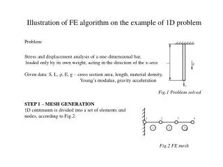
Illustration of FE algorithm on the example of 1D problem Problem: Stress and displacement analysis of a one-dimensional bar, loaded only by its own weight, acting in the direction of the x-axis Given data: S, L, r, E, g – cross section area, length, material density, Young’s modulus, gravity acceleration Fig.1 Problem solved STEP 1 – MESH GENERATION 1D continuum is divided into a set of elements and nodes, according to Fig.2. Fig.2 FE mesh
STEP 2 – DISPLACEMENT APPROXIMATION We concentrate now on the element no.1. Its displacement u(x) is approximated by linear shape functions Where is the shape function matrix, matrix of deformation parameters, which have a simple physical interpretation of displacements of mesh nodes - see Fig.3. Fig.3 Bar element
Linear shape functions where x1, x2are the nodal coordinates according to Fig.3. Displacement of any point of the bar is thus determined by displacement of its nodes as can be seen in Fig.4 Fig.4 Approximation of displacement
STEP 3 – ELEMENT STIFFNESS MATRIX From displacements, the approximation of strain and stress can be obtained, and where B is the matrix obtained from N by derivation or , if we denote the length of element as . Inserting stress and strain into the strain energy we obtain after some manipulations where k is the element stiffness matrix
STEP 4 – ELEMENT LOAD MATRIX By analogy, load matrix can be obtained inserting the displacement approximation into the potential of external forces , which results in . The load matrix represents total external loading of element (in this particular case its weight), localised into point forces acting in the nodes of the element. STEP 5 – GLOBAL STIFFNESS AND LOAD MATRIX Creating global matrix of deformation parameters , strain energy of the 1st element can be written
where is the stiffness matrix of the first element, enhanced by zero-element lines and columns to enable multiplication by the matrix U. By the same logic, stiffness matrices of the second and third element can be written as . As the total strain energy is a sum of element contributions, we can write it as , where K is the global stiffness matrix of the structure .
By the same procedure, global load matrix F can be obtained as a sum of element contributions to the total potential of external forces : , . STEP 6 – RESULTING SYSTEM OF EQUATIONS Using previous matrices K, F, total potential energy can be expressed as From the stationary condition
we obtain the system of four linear algebraic equations for the four deformation parameters u1, u2, u3, u4: . This is the basic equation to be solved. We can see that the stiffness matrix K is the matrix of coefficients. Detailed inspection of our K matrix shows, nevertheless, that it is singular and that the equations have thus no unambiguous solution. This is caused by the fact that we have not specified any boundary condition yet. We should remember a very important fact: In the static problems of displacement version of FEM, at least so many boundary conditions must be defined to prevent free motion of the analysed model. If this condition is not met, the resulting stiffness matrix is singular and solution of equations usually breaks down. To meet this condition in our case, we prescribe zero displacement for the first unknown, u1 = 0. This means that from the system of equations we must leave out the first equation, which results in the following form of our global matrices:
If we look at the structure of K matrix now, we can see it is a symmetric, positive definite band matrix with dominant diagonal, which is very helpful for quick, stable and efficient computational solution of very large systems of equations. STEP 7 – SOLUTION OF EQUATIONS Solution of the basic system of equations yields nodal displacements, from which the approximation of element displacement, strain and stress can be obtained according to the equations given above. Figs.5 and 6 show the difference between the analytical and numerical solution of this illustrative example. We should note, that the exact correspondence of numerical and analytical solution in nodal displacements is only a consequence of a very simple problem, it cannot be generalized. Typical for the elements with linear shape functions is, of course, linear approximation of displacements, and constant approximation of stress and strain on elements, with no continuity between elements - see Fig.6.
Fig.5 Displacements of bar Fig.6 Stress in the bar