Normal Distribution, Statistical Inference, Central Limit Theorem

1. Normal Distribution, Statistical Inference, Central Limit Theorem

2. What is the area under a normal distribution? • A. 100 • B. 1 • C. bimodal • D. depends on the conditional probabilities

3. Which of the following is a normal distribution? C A A B B D C D E. All of the above

4. How many standard deviations do you have to be above the mean to be accepted into Mensa? • A. about 100 • B. 1 • C. about 2 • D. depends on the test

5. What score can you use to compare students who have taken different tests? • A. an SAT score • B. an ACT score • C. You can’t compare tests like the ACT to tests like the SAT • D. a Z score

6. How confident are we that the mean of the same will approximate the population mean, given the following sampling distributions… • A distribution that looks like A versus B? B A

7. What else would that depend on?

8. The Normal Distribution

9. The Normal Distribution • Symmetric • Continuous = prob of any one point = zero, because the area of a line is zero – we always compute probabilities of lying between some designated x and y • All have same general shape • Cases more concentrated in the middle than in the tails • Shape determined by: mean and standard deviation • The area under the curve is 1 • The probability of any event under the curve is determined by the height of the curve at that place Number of cases = y axis Value of the variable = x axis

10. Why do we care about the Normal Distribution? 1) Many of the political phenomena that we study are distributed normally. For example, Ideology – there are lots of people in the middle and not as many people on the tails 2) The normal distribution has some cool properties, like being able to easily compute percentiles.

11. Approximately 68 percent of the area under a normal curve lies between the values of the mean and the standard deviation + and – the mean.

12. Approximately 95% of the area lies between 2 standard deviations + and – the mean.

13. Approximately 99.7% lies between 3 standard deviations + and – the mean.

14. Assume grades on a test are normally distributed mean of 80 standard deviation of 5 What is the percentile rank of a person who received a score of 70 on the test?

15. Z table

16. To take another example, what is the percentile rank of a person receiving a score of 90 on the test?

17. If a test is normally distributed with a mean of 60 and a standard deviation of 10, what proportion of the scores are above 85? A z table can be used to calculate that .9938 of the scores are less than or equal to a score 2.5 standard deviations above the mean. It follows that only 1-.9938 = .0062 of the scores are above a score 2.5 standard deviations above the mean. Therefore, only .0062 of the scores are above 85. Given the sample, what is the probability of selecting out a test grade higher than 85?

18. The Standard Normal Distribution Same as a normal distribution, but the standard deviation is 1 and the mean is 0 0

19. Any normal distribution can be turned into a standard normal with a linear transformation: 1) Subtract the mean from every observation 2) Divide by the standard deviation This is called a z-score.

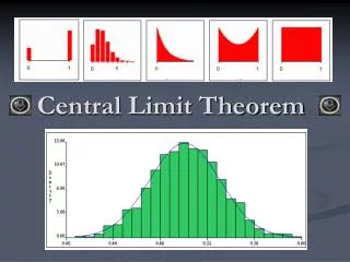
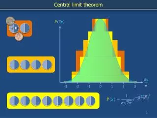
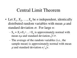
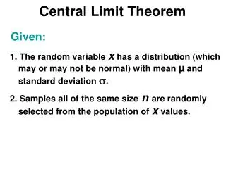
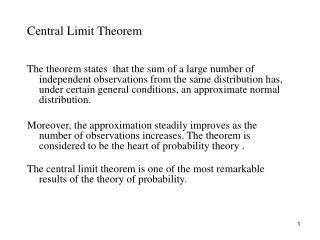
20. The Central Limit Theorem Given a population with ANY distribution: Taking random samples of size n from that distribution The sample means will be (approximately) normally distributed.

21. Sampling Distribution Illustration http://onlinestatbook.com/stat_sim/sampling_dist/ http://vimeo.com/75089338

22. Now, back to statistical analysis

23. Properties of Estimators Remember that Ordinary Least Squares minimizes the squared errors from the line.

24. Residuals 6 5 Slope 4 Political Tolerance Mean 3 2 1 0 0 1 2 3 4 5 6 Education

25. Residuals of OLS analysis (errors of the slope) have a mean of zero, by definition – they have been computed by their minimization. We also assume that they are distributed normally.

26. Residuals and OLS • Therefore they are distributed along a standard normal distribution, mean of zero. • The standard deviation is not necessarily 1, but it is assumed to be constant across all values of x. • Foreshadowing: if this assumption does not hold, you are not advised to use OLS.

27. Residuals are variables For each observation, they represent the squared distance from the slope.

28. What is the question that we ask with bivariate regression? • Is the slope different from the mean • If the slope = mean, then the slope = 0 • Is the slope zero? • The null hypothesis is that the slope is zero.

29. The Null Hypothesis Answer: How likely is it that the relationship is zero? The null hypothesis is that the relationship is zero. We are trying to reject the null hypothesis.

30. The Null Hypothesis We have a point estimate of y for each value of x We call it a slope, and tell what the points are on the slope, but we cannot be sure about that point because we do not know anything about the population. So, we know that there is error in our estimate. We put bounds around that estimate. So, to reject the null hypothesis, neither the upper nor lower bound of our estimate can contain zero.

31. Generally, we want to be at least 95% confident that our estimate does not include zero. 0 So, to be 95% confident that the true estimate does not contain zero, then the estimate must be two standard deviations from the mean of the standard normal curve, which is zero.

32. Instead, I am 95% confident that a confidence interval “covers” the true value from the population, based not on this single CI from this single test, but rather as a result of what would happen were I to repeat the process of drawing samples and doing this test over and over again.

33. If a certain interval is a 95% confidence interval, then we can say that if we repeated the procedure of drawing random samples and computing confidence intervals over and over again, 95% of those confidence intervals include the true value from the population. This is not to say that we are 95% confident that the true value lies between the upper and lower bound.