Download
1 / 97
980 likes | 1.01k Views
Learn about the characteristics, calculations, and applications of the normal distribution, central limit theorem, and statistical inference in this comprehensive guide.

E N D
The Normal Distribution, Central Limit Theorem, and Introduction to statistical inference
The Normal Distribution • ‘Bell Shaped’ • Symmetrical • Mean, Median and Mode are Equal m=mean s = standard deviation The random variable has an infinite theoretical range: + to p(X) s X m Mean = Median = Mode
Examples: • height • weight • age • bone density • IQ (mean=100; SD=15) • SAT scores • blood pressure • ANYTHING YOU AVERAGE OVER A LARGE ENOUGH # (Central Limit Theorem)
This is a bell shaped curve with different centers and spreads depending on and The Normal Distribution:as mathematical function (pdf) Note constants: =3.14159 e=2.71828
The 68-95-99.7 rule only gets you so far… • For example, what’s the probability of getting a math SAT score below 575 if SAT scores are normally distributed with a mean of 500 and a std dev of 50?? Solve this ... ?!
The Standard Normal Curve:“Universal Currency” All normal distributions can be converted into the standard normal curve by subtracting the mean and dividing by the standard deviation: For example, 575 in math SAT units translates to 1.5 standard deviations above the mean.
The Standard Normal Curve:“Universal Currency” Z~Normal(=0, =1)
The Standard Normal Distribution (Z) Somebody calculated all the integrals for the standard normal and put them in a table! So we never have to integrate! Even better, computers now do all the integration.
Comparing X and Z units 500 575 X ( = 500, = 50) 0 1.5 Z ( = 0, = 1)
Example So, What’s the probability of getting a math SAT score of 575 or less, =500 and =50? No need to do the integration! Just look up Z= 1.5 in standard normal chart no problem! = .9332
Z=1.50 Z=1.50 Looking up probabilities in the standard normal table What is the area to the left of Z=1.50 in a standard normal curve? Area is 93.32%
Exercise (in groups of 2-3) If birth weights in a population are normally distributed with a mean of 109 oz and a standard deviation of 13 oz, • What is the chance of obtaining a birth weight of 141 oz or heavier when sampling birth records at random? • What is the chance of obtaining a birth weight of 120 or lighter?
Answer • What is the chance of obtaining a birth weight of 141 oz or heavier when sampling birth records at random? From the chart Z of 2.46 corresponds to a right tail (greater than) area of: P(Z≥2.46) = 1-(.9931)= .0069 or .69 %
Answer b. What is the chance of obtaining a birth weight of 120 or lighter? From the chart Z of .85 corresponds to a left tail area of: P(Z≤.85) = .8023= 80.23%
Are my data “normal”? • Not all continuous random variables are normally distributed!! • It is important to evaluate how well the data are approximated by a normal distribution
Are my data normally distributed? • Look at the histogram! Does it appear bell shaped? • Compute descriptive summary measures—are mean, median, and mode similar? • Do 2/3 of observations lie within 1 std dev of the mean? Do 95% of observations lie within 2 std dev of the mean? • Look at a normal probability plot—is it approximately linear? • Run tests of normality (such as Kolmogorov-Smirnov). But, be cautious, highly influenced by sample size!
Example: Class coffee drinking (n=21) Mean=3.6 ounces/day Std Dev=5.1 ounces/day Range: 0 to 16
-1.5 8.7 Example: Class coffee drinking (n=21) Mean1 Std Dev= 3.6 5.1 = -1.5 to 8.7 (covers 90% of observations)
-6.6 13.8 Example: Class coffee drinking (n=21) Mean2 Std Dev= 3.6 10.2 = -6.6 to 13.8 (covers 90% of observations)
Normal Probability Plot Clearly not a straight line! Kolmogorov-Smirnov test agrees, not normal!
Example: Class wake-up times (n=20) Mean=7:20 Std Dev=0:56 Range: 5:00 to 9:00
8:16 6:24 Example: Class wake-up times (n=20) Mean1 Std Dev= 7:20 :56 = 6:24 to 8:16 (covers 80% of observations)
Example: Class wake-up times (n=20) Mean2 Std Dev= 7:20 1:52 = 5:28 to 9:12 (covers 95% of observations)
Normal Probability Plot Pretty close to a straight line! Kolmogorov-Smirnov test agrees, looks normal!
Review Problem 1 Which of the following about the normal distribution is NOT true? • Theoretically, the mean, median, and mode are the same. • About 2/3 of the observations fall within 1 standard deviation from the mean. • It is a discrete probability distribution. • Its parameters are the mean, , and standard deviation, .
Review Problem 1 Which of the following about the normal distribution is NOT true? • Theoretically, the mean, median, and mode are the same. • About 2/3 of the observations fall within 1 standard deviation from the mean. • It is a discrete probability distribution. • Its parameters are the mean, , and standard deviation, .
Review Problem 2 For some positive value of Z, the probability that a standard normal variable is between 0 and Z is 0.3770. The value of Z is: • 0.18. • 0.81. • 1.16 • 1.47.
Review Problem 2 For some positive value of Z, the probability that a standard normal variable is between 0 and Z is 0.3770. The value of Z is: • 0.18. • 0.81. • 1.16 • 1.47.
Review Problem 3 The probability that a standard normal variable Z is positive is ________. • 50% • 100% • 0% • 95%
Review Problem 3 The probability that a standard normal variable Z is positive is ________. • 50% • 100% • 0% • 95%
Review Problem 4 Suppose Z has a standard normal distribution with a mean of 0 and a standard deviation of 1. The probability that Z values are larger than __________ is 0.6985. • 1.0 • 0 • -0.6 • +0.6 • -2.0
Review Problem 4 Suppose Z has a standard normal distribution with a mean of 0 and a standard deviation of 1. The probability that Z values are larger than __________ is 0.6985. • 1.0 • 0 • -0.6 • +0.6 • -2.0
Statistical Inference: Hypothesis Testing and Confidence Intervals
What is a statistic? • A statistic is any value that can be calculated from the sample data. • Sample statistics are calculated to give us an idea about the larger population.
Examples of statistics: • mean • The average cost of a gallon of gas in the US is $2.87. • difference in means • The difference in the average gas price in San Francisco ($3.37) compared with Minneapolis ($2.65) is 72 cents. • proportion • 67% of high school students in the U.S. exercise regularly • difference in proportions • The difference in the proportion of men who approve of George W. (44%) and women who do (38%) is 6%
What is a statistic? • Sample statistics are estimates of population parameters.
Sample statistic: mean IQ of 5 subjects Truth (not observable) Sample (observation) Mean IQ of some population of 100,000 people =100 Make guesses about the whole population Sample statistics estimate population parameters:
Sampling Distributions Most experiments are one-shot deals. So, how do we know if an observed effect from a single experiment is real or is just an artifact of sampling variability (chance variation)? **Requires a priori knowledge about how sampling variability works… Question: Why have I made you learn about probability distributions and about how to calculate and manipulate expected value and variance? Answer: Because they form the basis of describing the distribution of a sample statistic.
What is sampling variation? • Statistics vary from sample to sample due to random chance. • Example: • A population of 100,000 people has an average IQ of 100 (If you actually could measure them all!) • If you sample 5 random people from this population, what will you get?
Truth (not observable) Sampling Variation Mean IQ=100
Sampling Variation and Sample Size • Do you expect more or less sampling variability in samples of 10 people? • Of 50 people? • Of 1000 people? • Of 100,000 people?
Standard error • Standard error is the standard deviation of a sample statistic. • It’s a measure of sampling variability.
What is statistical inference? • The field of statistics provides guidance on how to make conclusions in the face of this chance variation.
Examples of Sample Statistics: Single population mean (known ) Single population mean (unknown ) Single population proportion Difference in means (ttest) Difference in proportions (Z-test) Odds ratio/risk ratio Correlation coefficient Regression coefficient …
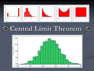
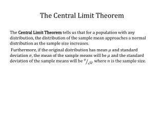
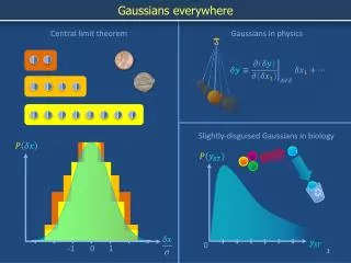
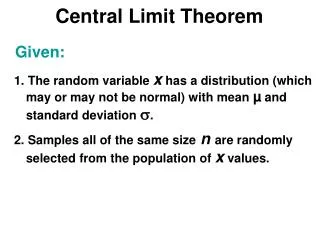
1. have mean: 2. have standard deviation: The Central Limit Theorem: If all possible random samples, each of size n, are taken from any population with a mean and a standard deviation , the sampling distribution of the sample means (averages) will: 3. be approximately normally distributed regardless of the shape of the parent population (normality improves with larger n)
The mean of the sample means. The standard deviation of the sample means. Also called “the standard error of the mean.” Symbol Check