Download

1 / 58
580 likes | 734 Views
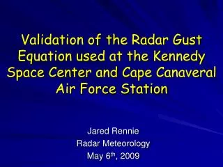
Evaluation of WSR-88D Methods to Predict Warm Season Convective Wind Events at Cape Canaveral Air Force Station and Kennedy Space Center. Jared Rennie Thesis Defense February 26 th , 2010. Overview. Introduction and Background Data and Methodology Results Verification of Existing Methods

E N D
Evaluation of WSR-88D Methods to Predict Warm Season Convective Wind Events at Cape Canaveral Air Force Station and Kennedy Space Center Jared Rennie Thesis Defense February 26th, 2010
Overview • Introduction and Background • Data and Methodology • Results • Verification of Existing Methods • New Methods: Regression Based • New Methods: CART based • Final Notes • Questions
Convective Wind Events • Hard to accurately predict • Small spatial resolution • Short lifecycles • Large variability • Major hazards for processing space vehicles and payloads for launch • Cape Canaveral Air Force Station (CCAFS) • Kennedy Space Center (KSC)
45th Weather Squadron • Responsible for predicting convective winds on the CCAFS/KSC complex • Warnings (surface – 300 ft AGL) • ≥ 35 kt with desired lead time of 30 minutes • ≥ 50 kt with desired lead time of 60 minutes • Categorize downburst prediction into a four step funnel process
Examples of Nowcasting Methods Regression based radar gust equations VIL = Vertically integrated liquid ET = Echo tops (18 dBZ) MaxZ = Maximum reflectivity Height = Height of the maximum reflectivity Stewart’s (1996) ET/VIL Equation Loconto’s (2006) Radar Gust Equation
Examples of Nowcasting Methods Relationship between cell’s maximum reflectivity and RAOB defined freezing level (Loconto 2006)
Issues • Small sample size used in previous studies • Onset • Cases only used data at or just before the time of the reported wind gust • Ideal if techniques were correlated with previous volume scans in order to provide a longer lead time to the forecaster
Objectives • Evaluate previous methods with an expanded dataset for onset and earlier volume scans • Introduce new techniques in hopes to improve decision making when nowcasting a convective wind event • GOAL: maximize the True Skill Statistic that finds the optimum compromise between the Probability of Detection and Probability of False Alarm
Data • 2003 – 2009 • Peak wind gusts from weather towers on CCAFS/KSC complex • Events above AND below 35 knots • Considered “true values” for research • KXMR RAOB freezing level heights
Data • 2003-2009 • NCDC Storm Structure Data Files • Cell based vertically integrated liquid [kg m-2] • Echo top [kft] • Maximum reflectivity [dBZ] • Height of maximum reflectivity [kft] • VIL Density = VIL[kg m-3] ET Gathered for onset, and four volumetric scans prior
Data Warning cell has boundary interaction 70% of time Non-warning cell has no boundary interaction 65% of the time • 2003-2009 • Radar Summary Data • Categorical data that provides information about a gust producing convective cell • Cell Type • Cell Strength • Boundary Interactions • Group Movement • Individual Cell Movement • Location of Peak Wind (Ander et al. 2009)
Verification of Existing Methods • Radar Gust Equations • Scatterplots between predicted and observed peak wind gusts • Fitted Regression Line • Correlation Coefficient (R2 value) • Forecast Errors • Root Mean Square Error (RMSE) • Mean Absolute Error (MAE) • Number of hits (within ± 5 kt of Accuracy) • Percentage of Hits
Verification of Existing Methods • Relationship between height of maximum reflectivity and freezing level • Provide similar plots • 2X2 contingency tables
Introduction of New Methods • Partition of dataset • Training set to BUILD model: 2003-2007 • Independent set to TEST model: 2008-2009 • All models generated in the R statistical environment
Regression Models • Multiple Linear Regression • Used to create NEW radar gust equations • Variable Selection • RESPONSE: Recorded wind gust • PREDICTORS: VIL, VIL Density, Echo Top, Max Reflectivity, Height of Max Reflectivity
Regression Models • Logistic Regression • Does not assume normality of data • Assumes binary response • RESPONSE: Episode 0 = Gust < 35 kt 1 = Gust ≥ 35 kt • PREDICTORS: Same as MLR with addition of Boundary Interactions
Verification of Regression Models • Multiple linear regression • Scatterplots of predicted vs. observed gust • Forecast Errors • Logistic regression • 2X2 Contingency Tables • Calculate performance metrics • Probability of Detection (POD) • Probability of False Alarm (POFA) • True Skill Statistic (TSS)
Classification and Regression Trees (CART) • Provides objective forecasts without the parametric assumptions of the relationship between the response and predictors • Stratifies data into categories and provides yes/no decision branches (nodes) to classify future events into the most likely branch • RESPONSE: Episode 0 = Gust < 35 kt 1 = Gust ≥ 35 kt • PREDICTORS: VIL, VIL Density, Echo Top, Max reflectivity, height of max reflectivity, boundary interactions
CART • Advantages • Can handle large datasets • Does not need variable selection • Can handle outliers and non-linear relationships • Easy to implement, train, and automate • Disadvantages • Reasons for tree branching may be unclear • Tree can be over fitted with too many leaves and too many end nodes
Five Tree Algorithms Used • Each unique and handles data differently • Some methods are user-friendly • Some methods have higher performance • Recursive Partitioning and Regression • Conditional Inference • Bootstrap Aggregation • Boosting • Random Forests
Verification of CART models • Use independent dataset to run through the trees and output a 0 or 1 • 0 = Cell will produce a wind gust < 35 kt • 1 = Cell will produce a wind gust ≥ 35 kt • Construct 2X2 contingency table • Calculate performance metrics • POD, POFA, TSS
Performance Metrics • What we would like to see • High POD’s • Low POFA’s • TSS > 0.3 (Wilks 2005)
Results Number of Cases
Verification of Previous Methods Introduction of New Methods
Results Verification of Existing Methods
Radar Gust Equations • Scatter Plots • Scatter across all of the graphs • Low correlation coefficients • ET/VIL equation: 0.14 – 0.17 • Loconto equation: 0.16 – 0.20 • Fitted regression lines contain slope < 1 and large non-zero intercepts • Under predicts weak gusts • Over predicts strong gusts
Radar Gust Equations • Forecast Errors
Height of Max Reflectivity vs. Freezing Level Relationship • Plots • Similar to previous analysis • Positive Height Difference = Gust ≥ 35 kt • Negative Height Difference = Gust < 35 kt • Different • Linear increase in maximum reflectivity versus peak wind gust • Correlation coefficients between 0.42 and 0.65
Height of Max Reflectivity vs. Freezing Level Relationship • Performance Metrics
Summary • Radar gust equations do not perform as well as earlier results indicated • RMSE and MAE values too high • Correlation coefficients and hit rates too low • Relationship between height of max reflectivity and freezing level has less validity • May be a relationship between reflectivity and peak gust • Not looked into any further
Results New Methods: Regression Based
Summary • Multiple Linear Regression Models • Do not perform well against independent dataset • High RMSE and MAE values • Logistic Regression Models • Positive performance
Results New Methods: CART Based
Recursive Partitioning and Regression Trees (rpart) • Basic CART producer in R • Splits sample into smaller subgroups based on the purity of the response • Recursive partitioning continues until stopping criterion is met • Pruning may be performed through the cost-complexity parameter (Therneau and Atkinson 1997)
rpart • Settings can be adjusted by the user • Depth of the tree • How many splits are made • Cost Complexity parameter • Models stratified by volumetric scan • Built using test set from 2003-2007 • Tested using independent set from 2008-2009
Performance of rpart a = cell initiated by neither SBF or OFB
Conditional Inference Trees (ctree) • Uses hypothesis testing to prevent over fitting of the tree • P-values generated for each candidate predictor • If lowest p-value is below significant threshold (0.05) then a split will occur • Tree is grown until no more nodes have a statistically significant relationship • Pruning is not required (Hothorn et al. 2006)
Bootstrapping • Next three tree algorithms uses technique called bootstrapping • Random sampling with replacement is performed on original dataset • Creates multiple subsets of data • NOT independent of each other • Statistical test is applied to each subset • Analogous to ensemble models in NWP • Can reduce the variance of predictions, however can be computationally intensive (Wilks 2005)
Bootstrap Aggregation (bagging) • Creates 100 re-samples of data and produces 100 trees • Trees generated through rpart algorithm • Final classification is determined by popular vote • Trees not shown, however can provide variable importance • Percentage of how many times predictor is used for splitting (Breiman 1996)
Boosting • Creates 100 re-samples of data and produces 100 trees using rpart defaults • Creates adjusted weights of original dataset after each iteration instead of random selection • Final classifications determined by a weighted vote of the iteratively produced classifiers (Freund and Schapire 1996)
Random Forests • Build a collection of de-correlated trees • Determines final classification by popular vote over the ensemble of trees • 500 trees are generated • Variable importance not calculated by percentage of use, but rather the mean decrease Gini • Total decrease in node impurities from splitting on the variable, averaged over all of the trees (Breiman 2001)