CEE262C Lecture 3: The predator-prey problem
160 likes | 457 Views
CEE262C Lecture 3: The predator-prey problem. Overview. Lotka-Volterra predator-prey model Phase-plane analysis Analytical solutions Numerical solutions References: Mooney & Swift, Ch 5.2-5.3;. Compartmental Analysis. Tool to graphically set up an ODE-based model Example: Population.

CEE262C Lecture 3: The predator-prey problem
E N D
Presentation Transcript
CEE262C Lecture 3: The predator-prey problem Overview • Lotka-Volterra predator-prey model • Phase-plane analysis • Analytical solutions • Numerical solutions References: Mooney & Swift, Ch 5.2-5.3; CEE262C Lecture 3: Predator-prey models
Compartmental Analysis • Tool to graphically set up an ODE-based model • Example: Population Immigration: ix Emigration: ex Population: x Births: bx Deaths: dx CEE262C Lecture 3: Predator-prey models
Logistic equation Population: x Can flow both directions but the direction shown is defined as positive CEE262C Lecture 3: Predator-prey models
Income class model Lower x Middle y Upper z CEE262C Lecture 3: Predator-prey models
For a system the fixed points are given by the Null space of the matrix A. For the income class model: CEE262C Lecture 3: Predator-prey models
Classical Predator-Prey Model cxy bxy Predator y Prey x ax dy Growth in absence of predators Die-off in absence of prey Lotka-Volterra predator-prey equations CEE262C Lecture 3: Predator-prey models
Assumptions about the interaction term xy • xy = interaction; bxy: b = likelihood that it results in a prey death; cxy: c = likelihood that it leads to predator success. An "interaction" results when prey moves into predator territory. • Animals reside in a fixed region (an infinite region would not affect number of interactions). • Predators never become satiated. CEE262C Lecture 3: Predator-prey models
Phase-plane analysis CEE262C Lecture 3: Predator-prey models
Analytical solution CEE262C Lecture 3: Predator-prey models
Solution with Matlab lvdemo.m % Initial condition is a low predator population with % a fixed-point prey population. X0 = [x0,.25*y0]'; % Decrease the relative tolerance opts = odeset('reltol',1e-4); [t,X]=ode23(@pprey,[0 tmax],X0,opts); pprey.m function Xdot = pprey(t,X) % Constants are set in lvdemo.m (the calling function) global a b c d % Must return a column vector Xdot = zeros(2,1); % dx/dt=Xdot(1), dy/dt=Xdot(2) Xdot(1) = a*X(1)-b*X(1)*X(2); Xdot(2) = c*X(1)*X(2)-d*X(2); CEE262C Lecture 3: Predator-prey models
at t=0, x=20 y=19.25 CEE262C Lecture 3: Predator-prey models
Nonlinear Linear CEE262C Lecture 3: Predator-prey models