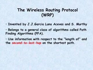
The Wireless Routing Protocol (WRP)
The Wireless Routing Protocol (WRP). Invented by J.J.Garcia Luna Aceves and S. Murthy Belongs to a general class of algorithms called Path Finding Algorithms (PFA). Use information with respect to the “length of†and the second-to-last-hop on the shortest path. Path Finding Algorithm.

The Wireless Routing Protocol (WRP)
E N D
Presentation Transcript
The Wireless Routing Protocol (WRP) • Invented by J.J.Garcia Luna Aceves and S. Murthy • Belongs to a general class of algorithms called Path Finding Algorithms (PFA). • Use information with respect to the “length of” and the second-to-last-hop on the shortest path.
Path Finding Algorithm • Each node maintains the shortest path spanning tree maintained by each of its neighbors. • Using this, it creates its own shortest path spanning tree. • Note: Shortest path Shortest Weighted Path • Periodically, each node broadcasts an update (could be null: why?) that reports updates to its spanning tree. • Each update contains : • The destination address • Distance to that destination • An identifier of the node that is at the second-to-last-hop on the shortest path to that destination.
WRP : Nitty Gritty Details • Uses the generic ideas in PFA • Reduces the number of “temporary” routing loops. • Let us call “second-to-last-hop” node as the predecessor node. • When a node receives an update from a neighbor it checks the “consistency ” of the predecessor information reported by all its neighbors. • The spanning tree also gives info with regards to the next hop neighbor towards that destination. We call this next hop neighbor the successor node.
In WRP, each node maintains four tables: • Distance Table • Routing Table • Link-Cost Table • Message Retransmission List (MRL)
Distance Table • Let us consider a particular node A. • In this table, for each destination K, node A maintains the distance to K via each of its neighbors (say B) DAKB, and the predecessor node PAKB, along that path. • This table is used in the construction of the minimum spanning tree.
Routing Table • Aided by the spanning tree formed: thanks to the distance table. • For each destination Node K, it contains • The address of Node K. • The distance to Node K. • The successor on the shortest path to Node K. • The predecessor on this path to Node K. • May also contain a flag to indicate whether the path is correct, or erroneous (no path to destination).
Link-Cost Table • Tabulates the cost of transmitting through each neighbor. • Note : Cost depends on link characteristics – need not be hop count. • Also contains for each neighbor B, the time that has elapsed since last receiving an error free message from B.
Message Re-transmission List • Contains info with regards to each transmitted update by the node (say node A). • Each update message has a seq. no. that is tabulated in this table. • Also contains a retransmission counter and ACK required flag vector. • The flag vector indicates the neighbors that responded to the update. • Help eliminate redundant update transmissions.
WRP: An Example Let cost of Link 2 be ’10’. ROUTING TABLE AT A
Now Let Link 1 fail. • Node A will notice this failure. • Let us consider a single destination – say Node X. • Node A will set the distance to X to infinity and its predecessor and successor values to “null”. • This is broadcast to Node C. • Node C computes the alternate route to A which is by means of Link 2. • This info is then transmitted to A. • A then realizes (by means of C’s new spanning tree) that it can reach other nodes via C.
Advantages/ Limitations • Advantages: • No Loops • Lower number of updates upon link failure – reports sent only to neighbors. • Overhead grows as O(n) – n is the number of nodes. • Disadvantages • Messages may be large. • Maintenance of four tables. • Hello packets required – cannot go into sleep mode – overhead. • Scalability still an issue !
Reference • E.M. Royer and C-K.Toh, “A Review of Current Routing Protocols for Ad Hoc Wireless Networks”, IEEE Personal Communications Magazine, pp 46-55, April 1999. • S.Murthy and J.J.Garcia-Luna-Aceves, “An Efficient Routing Protocol for Wireless Networks”, ACM Mobile Networks and Applications Journal, pp 183-197, October 1996. • http://www.cse.ucsc.edu/research/ccrg/
Link State Routing • Distance Vector Routing Protocols are attractive because of their simplicity. • Another class of protocols that are “proactive” (exchange control messages to form and maintain routing tables even before they are required) are “link state routing “ protocols. • Popular Link State Routing Protocol -- OSPF • Require each and every node in the network to have a knowledge of the complete topology of the network. • A local computation of the best path to each destination is made.
D A Link 2 Link 4 C Link 1 Link 6 B Link 3 Link 5 E The Network is now depicted by the Map shown as
A particular node is responsible for each entry of this table. • It has to update this periodically. • Update is to be relayed to all nodes in the network. • The entry termed as “cost” is also often referred to as “state”. • Once each node has the entire topology map, it tries to compute the shortest path to each destination. • Can you think of one popular algorithm that is used for achieving this ?
YES! It is the Dijkstra’s Algorithm. • Each node computes shortest “weighted” path tree using this topology information; it places itself at the root of this tree. • Reference : “Introduction to Algorithms” by Cormen, Leiserson and Rivest.
ADVANTAGES: • Each node can do a local “loop free” computation. • Can reflect appropriate metrics to reflect the “state” of a link. • DISADVANTAGES • Not scalable • Each link state update has to be “flood” to every node in the network – flooding is expensive – especially in an ad hoc network where link-state changes are frequent. • Note: Sequence numbers are required to ensure that flooding does not continue for ever !