Data Quality and Rule Discovery in Classification
Explore the principles of data quality, decision trees, and association rules in classification projects. Learn to parse files, generate tables, and identify key patterns. Discover CART, selection heuristics, and association rule algorithms for effective data analysis.


Data Quality and Rule Discovery in Classification
E N D
Presentation Transcript
Data Quality Class 9
Agenda • Project – 4 weeks left • Exam – • Rule Discovery • Data Linkage
Project • Please email me a schema by Friday • I will review the schema • By next Friday: • Application to parse a file and generate table entries
Exam • Answers to questions
Rule Discovery • Decision and ClassificationTrees • Association Rules
Decision and Classification Trees • Each node in tree represents a question • Decision as to which path to take from that node is dependent on the answer to the question • At each step along the path from the root of the tree to the leaves, the set of records that conform to the answers along the way continues to grow smaller
Decision and Classification – 2 • At each node in the tree, we have a representative set of records that conform to the answers to the questions along that path • Each node in the tree represents a segmenting question, which subdivides the current representative set into two smaller segments • Every path is unique • Each node in the tree also represents the expression of a rule
CART • Classification and Regression Tree • Grab a training set • Subselect some records that we know already share some attribute properties in common • All other data attributes become independent variables • The results of the decision tree process are to be applied to the entire data set at a later date
CART 2 • Decide which of the independent variables is the best for splitting the records • The choice for the next split is based on choosing the criteria that divide the records into sets where, in each set, a single characteristic predominates • Evaluate the possible ways to split based on each independent variable, measuring how good that split will be
Selection Heuristics • Gini: maximize the set differentiated by a split, with the goal of isolating records with that class from other records • Twoing: tries to evenly distribute the records at each split opportunity • There are other heuristics
CART 3 • The complete tree is built by recursively splitting the data at each decision point in the tree • At each step, if we find that for a certain attribute all values are the same, we eliminate that attribute from future consideration • When we reach a point where no appropriate split can be found, we determine that node to be a leaf node • When the tree is complete, the splitting properties at each internal node can be evaluated and assigned some meaning
Rules • If (monthly_bill > 100) AND (PayPerViews < 2) • If (monthly_bill > 100) AND (PerPerViews > 2) AND (PayPerViews < 5) • If (monthly_bill > 100) AND (PayPerViews >= 5)
Association Rules • Rules of the form X Y, where X is a set of (attribute, value) pairs and Y is a set of (attribute, value) pairs • An example is “94% of the customers that purchase tortilla chips and cheese also purchase salsa” • This can be used for many application domains, such as market basket analysis • Can also be used to discover data quality rules
Association Rules 2 • Formally: • Let D be a database of records • Each record R in D contains a set of (attribute, value) pairs (also called an item) • An itemset X is a subset of (attribute, value) pairs of a record R (i.e., X R) • An association rule is an implication of the form X Y, where X and Y are both itemsets, and share no attributes. • The rule holds with confidence c if c% of the records that contain X also contain Y • The rule has supports% if s% of the records in D contain X or Y
Association Rules 3 • Confidence is the percentage of time that the rule holds when X is in the record • Support is the percentage of time that the rule could hold • Association rules describe a relation imposed on individual values that appear in the data • Association rules with high confidence are likely to imply generalities about the data • We can infer data quality rules from the discovery of association rules
Association Rules 4 • Example: • (CustomerType==Business) AND (total > $1000) (managerApproval == “required”) with confidence 85% and support 25% • This means that 25% of the time, the record had one of those attributes set with the indicated values • Of the records with (CustomerType==Business) AND (total > $1000), 85% of the time he attribute managerApproval had the value “required” • We might infer this as a more general rule, that business orders greater than $1000 require manager approval • This calls into question the 15% of the time it didn’t hold true – data quality problem, or is it not a general rule?
Association Rules 5 • We can set some minimum support and minimum confidence levels • Definitions: • Lkis the set of large sets having k items • Ckis the set of candidate sets having k items
Association Rules Algorithm • L1= sets with 1 item • for (k = 2; Lk-1not empty; k++) do • Ck= generate_new_candidates(Lk-1) • forall records R in D do • CR = subset(Ck, R) • forall candidates c in CRdo • c.count++; • end • Lk= {c in CR| c.count > minimum support}
Candidate Generation and Subset • Takes the set of all large itemsets of size (k – 1) • First, it joins Lk-1 with Lk-1, if they share (k – 2) items, to get a superset of the set of candidates • The candidates are pruned if a subset of the items in each candidate does not have minimum support (i.e., the subset of size (k – 1) is not in Lk-1 • Subset operation takes a record, and finds all candidate rules of iteration k within that record
More on Association Rules • We can adjust our goals for finding rules by quantizing the values in each attribute • In other words, we can assign values of attributes that belong to large ranges into quantized components, making the rule process less cumbersome • We can also use clustering to ehnace the association rule algorithm • If we don’t know how to quantize to begin with, use clustering for values • Association rules can uncover interesting data quality and business rules
Record Linkage • Critical component of data quality applications • Linkage involves finding a link between a pair of records, either through an exact match or through an approximate match • Linkage is useful for • data cleansing • data correction • enhancement • householding
Record Linkage 2 • Two records are linked when they match with enough weighted similarity • Matching can be a combination of exact matching on particular fields, to approximat ematching with some degree of similarity • For example: two customer records can be linked via an account number, if account numbers are uniquely assigned to customers
Record Linkage 3 • Example: • David Loshin • 633 Evergreen Terrace • Montclair, NJ • 201-765-8293 vs. • H. David Loshin • 633 Evergreen • Montclair, NJ • 201-765-8293 • In this case, we can establish a link based solely on telephone number
Record Linkage 4 • Frequently, pivot attributes exists and can be used for exact matching (such as social security number, account number, telephone number, student ID) • Often, there is no pivot attribute, and therefore approximate matching techniques must be used • Approximate matching is a process of looking for similarity
Similarity • As with clustering, we use measures of similarity to establish measures and thresholds for linkage • Most interesting areas for similarity are in string matching
String Similarity • How do we characterize similarity between strings? • We can see it with our eyes, or hear it inside our heads: • example: Smith, Smythe • example: John and Mary Jones, John Jones • How do we transfer this to automation?
Edit Distance • Edit distance operations • Insertion, where an extra character is inserted into the string • Deletion, where a character has been removed from the string • Transposition, in which two characters are reversed in their sequence • Substitution, which is an insertion followed by a deletion
Edit Distance 2 • Strings with a small edit distance are likely to be similar • Edit distance is measured as a count of edit distance operations from one string to another: • internatianl • transposition • internatinal • insertion • international • internatianl to international has an edit distance of 2
Computing Edit Distance • Use dynamic programming • Given two strings, x = x1x2 .. xn, and y = y1y2 ..ym • the edit distance f(i, j) is computed as the best match of two substrings x1x2 .. xi and y1y2 ..yjwhere • f(0,0) = 0 • f(i, j) = min[f(i-1, j) + 1), f(i, j-1) +1, f(i-1, j-1) + d(xi,yj)]
Phonetic Similarity • Words that sound the same may be misspelled • Phonetic similarity reduces the complexity of the strings • Effectively, it compresses the strings, with some loss, then performs a similarity test
Soundex • The first character of the name string is retained, and then numbers are assigned to following characters • The numbers are assigned using this breakdown: • 1 = B P F V • 2 = C S K G J Q X Z • 3 = D T • 4 = L • 5 = M N • 6 = R • Vowels are ignored
Soundex – 2 • Examples: • Fitzgerald = F322 • Smith = S530 • Smythe = S530 • Loshin = L250
Soundex – 3 • Regular soundex is flawed • geared towards English names • can’t account for incorrect first letter • longer names are truncated • Options • encode entire string, not just the first 4 consonant sounds • reverse the words, then encode both forward and backward • Use different phonetic encodings
Other Phonetic Encoding • NYSIIS • Similar to soundex, but • does not use numeric encoding, instead uses mapping to smaller set of consonants • replaces all vowels with “A” • Metaphone • Tries to be more exact with multiple-letter sounds (sh, tio, th, etc.)
N-gramming • Another means of representing a “compressed” form of a string • An n-gram is a chunk of text of length n • We slide a window of size n across a string to generate the set of n-grams for that string
N-gram Example • INTERNATIONAL is comprised of these 2-grams: • IN, NT, TE, ER, RN, NA, AT, TI, IO,ON, NA, AL • Compare this with INTERNATIANL • IN, NT, TE, ER, RN, NA, AT, TI, IA, AN, NL • These two strings share 8 2-grams
N-gram Measures • 1) Absolute overlap – this is the absolute ratio of matching n-grams to the total number of n-grams. This is equal to (2 (|ngram(X) ngram(Y)|)) (|ngram(X)| + |ngram(Y)|) • 2) Source overlap – this is the number of matching n-grams divided by the number of n-grams in the source string X: (|ngram(X) ngram(Y)|) |ngram(X)| • 3) Search overlap: this is the number of matching n-grams divided by the number of n-grams in the search string Y: (|ngram(X) ngram(Y)|) |ngram(Y)|