Tracing Heliospheric Structures to Their Solar Origin Robert Wimmer-Schweingruber

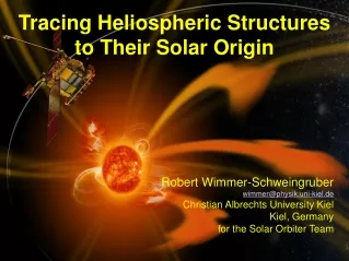
1. 2014 Fall AGU, San Francisco, 2014-12-17 Tracing Heliospheric Structures to Their Solar Origin Robert Wimmer-Schweingruber wimmer@physik.uni-kiel.de Christian Albrechts University Kiel Kiel, Germany for the Solar Orbiter Team

2. 2014 Fall AGU, San Francisco, 2014-12-17 Tracing Heliospheric Structures to Their Solar Origin The Problem What can we measure? Linkage... The End

3. 2014 Fall AGU, San Francisco, 2014-12-17 Remote-sensingwindows (10 days each) High-latitude Observations High-latitude Observations Perihelion Observations The Problem How does the Sun create and control the Heliosphere – and why does solar activity change with time ? 1) What drives the solar wind and where does the coronal magnetic field originate from? 2) How do solar transients drive heliospheric variability? 3) How do solar eruptions produce energetic particle radiation that fills the heliosphere? 4) How does the solar dynamo work and drive connections between the Sun and the heliosphere? Perihelion Observations High-latitude Observations

4. 2014 Fall AGU, San Francisco, 2014-12-17 Remote-sensingwindows (10 days each) High-latitude Observations High-latitude Observations Perihelion Observations What can we measure? Magnetic field on the Sun (PHI) Hydrogen density (EUI, METIS) Helium density (EUI) Composition on disk (SPICE) LOS flow velocities (SPICE, PHI) He/H in corona (EUI & METIS) Turbulence in corona (EUI, SoloHI) Eruptive events (EUI, METIS, PHI, SoloHI, STIX) Perihelion Observations High-latitude Observations

5. 2014 Fall AGU, San Francisco, 2014-12-17 Remote-sensingwindows (10 days each) High-latitude Observations High-latitude Observations Perihelion Observations What can we measure? EUI: Perihelion Observations High-latitude Observations

6. 2014 Fall AGU, San Francisco, 2014-12-17 Remote-sensingwindows (10 days each) High-latitude Observations High-latitude Observations Perihelion Observations What can we measure? EUI: Perihelion Observations High-latitude Observations

7. 2014 Fall AGU, San Francisco, 2014-12-17 Remote-sensingwindows (10 days each) High-latitude Observations High-latitude Observations SP+ Perihelion Observations What can we measure? EUI: Perihelion Observations High-latitude Observations

8. 2014 Fall AGU, San Francisco, 2014-12-17 Remote-sensingwindows (10 days each) High-latitude Observations High-latitude Observations Perihelion Observations What can we measure? Magnetic field on the Sun (PHI) Hydrogen density (EUI, METIS) Helium density (EUI) Composition on disk (SPICE) LOS flow velocities (SPICE, PHI) He/H in corona (EUI & METIS) Turbulence in corona (EUI, SoloHI) Eruptive events (EUI, METIS, PHI, SoloHI, STIX) Perihelion Observations High-latitude Observations

9. 2014 Fall AGU, San Francisco, 2014-12-17 Remote-sensingwindows (10 days each) High-latitude Observations High-latitude Observations Perihelion Observations What can we measure? Magnetic field on the Sun (PHI) Hydrogen density (EUI, METIS) Helium density (EUI) Composition on disk (SPICE) LOS flow velocities (SPICE, PHI) He/H in corona (EUI & METIS) Turbulence in corona (EUI, SoloHI) Eruptive events (EUI, METIS, PHI, SoloHI, STIX)

10. 2014 Fall AGU, San Francisco, 2014-12-17

11. 2014 Fall AGU, San Francisco, 2014-12-17 SPICE, EUI, and PHI high-res field of view at perihelion

12. 2014 Fall AGU, San Francisco, 2014-12-17 3% of disk at perihelion: - approx. 18 degrees as seen from Sun center - apparent solar rotation rate at perihelion is ~ 6°/day - thus, same source region remains in box for ~ 3 days - typical travel time: 60 rsun/400 km/s = 1.25 days - typical travel time: 60 rsun/300 km/s = 1.6 days Mapping the origin of the solar wind looks feasible if it comes the disk center. BUT: Does it? Well, that's what Solar Orbiter is all about.

13. 2014 Fall AGU, San Francisco, 2014-12-17 The problem lies in the super- radial expansion of flux tubes. This is well illustrated by the PFSS 'hairy-ball' model to the left and the coronal funnels shown below. Tu et al, 2005

14. Magnetograms from PHI Coronal Structure from EUI and METIS 2014 Fall AGU, San Francisco, 2014-12-17

15. 2014 Fall AGU, San Francisco, 2014-12-17 The Third “Instrument”: Models For instance map solar wind back to coronal & chromospheric origin (Peleikis et al., SH31B-03 Kruse et al., SH13A-4080)

16. 2014 Fall AGU, San Francisco, 2014-12-17 The Third “Instrument”: Models For instance map solar wind back to coronal & chromospheric origin (Peleikis et al., SH31B-03 Kruse et al., SH13A-4080)

17. 2014 Fall AGU, San Francisco, 2014-12-17 The Third “Instrument”: Models For instance map solar wind back to coronal & chromospheric origin Assumes constant speed from source to observation! - Horbury and Matteini (SH21B-4097) (Peleikis et al., SH31B-03 Kruse et al., SH13A-4080)

18. 2014 Fall AGU, San Francisco, 2014-12-17 The Third “Instrument”: Models For instance map solar wind back to coronal & chromospheric origin Assumes constant speed from source to observation! - Horbury and Matteini (SH21B-4097) - Weber and Kasper (SH12A-08) - Kruse et al. (SH31A-4080) (Peleikis et al., SH31B-03 Kruse et al., SH13A-4080)

19. 2014 Fall AGU, San Francisco, 2014-12-17 Solar Orbiter works best with all instruments together SO & SP+ SO & SP+ PHI, EUI, STIX, SPICE RPW METIS, Solo-HI MAG, SWA SO SO EPD EUI STIX IUGG/IAGA 2011 Session A101 - July 2/3

20. 2014 Fall AGU, San Francisco, 2014-12-17 Processes that affect solar wind composition: Some of these processes can be modeled. Providing simple models, e.g., for FIP, charge states, etc. would be very helpful.

21. 2014 Fall AGU, San Francisco, 2014-12-17 SPICE will provide Doppler-maps for various ions (SOHO/SUMER)

22. 2014 Fall AGU, San Francisco, 2014-12-17 Outflow along flux tubes (from coronal models) Composition (low/high FIP) also from SPICE, compare with SWA (SOHO/SUMER)

23. 2014 Fall AGU, San Francisco, 2014-12-17 Charge states are continuously modified by ionization and re-combination. Both are proportional to coronal electron density. Bochsler, 2007

24. 2014 Fall AGU, San Francisco, 2014-12-17 Charge states freeze in in the solar wind expansion process In situ charge states have lost all memory of what happened in deep corona. They retain memory of their last charge modification (charge states frozen in) in the upper corona.

25. 2014 Fall AGU, San Francisco, 2014-12-17 Charge-state and elemental composition somehow linked. Slow wind hot (source?) Fast wind cool (coronal hole) What links chromosphere and corona? Slow wind strongly FIPped Fast wind weakly/barely FIPped Geiss et al.1995)

26. 2014 Fall AGU, San Francisco, 2014-12-17 Individual streams can be identified in-situ by many independent methods: - magnetic field - plasma data - specific entropy - composition Composition is not altered by kinetic processes and remains conserved once it has been set in chromosphere and corona. Excellent tracer! Composition variable, especially in slow wind.

27. 2014 Fall AGU, San Francisco, 2014-12-17 Composition remains frozen in, i.e., does not change and therefore can be measured at 1 AU. Expect enhanced time dependence, but also less washing out of kinetic properties. Cleaner boundaries! Solar Orbiter will go here! STEREO/HI

28. 2014 Fall AGU, San Francisco, 2014-12-17 Charge-state and elemental composition somehow linked. Slow wind hot (source?) Fast wind cool (coronal hole) What links chromosphere and corona? Slow wind strongly FIPped Fast wind weakly/barely FIPped Geiss et al.1995)

29. 2014 Fall AGU, San Francisco, 2014-12-17 Charge-state and elemental composition somehow linked. Slow wind hot (source?) Fast wind cool (coronal hole) What links chromosphere and corona? Brooks and Warren, 2011 Slow wind strongly FIPped Fast wind weakly/barely FIPped Geiss et al.1995)

30. 2014 Fall AGU, San Francisco, 2014-12-17 Origin of the Slow Solar Wind? Edges of Coronal holes Edges of Active regions S-web (coronal hole extensions provide open field connection) Interchange reconnection

31. 2014 Fall AGU, San Francisco, 2014-12-17 Solar Orbiter works best with all instruments together SO & SP+ SO & SP+ PHI, EUI, STIX, SPICE RPW METIS, Solo-HI MAG, SWA SO SO EPD EUI STIX IUGG/IAGA 2011 Session A101 - July 2/3

32. 2014 Fall AGU, San Francisco, 2014-12-17 Information from EPD 3He is preferentially accelerated in flares (probably wave-particle interaction) → flare origin! Velocity dispersion indicates rapid acceleration and good connection → no time for diffusion!

33. 2014 Fall AGU, San Francisco, 2014-12-17 Information from EPD Velocity dispersion also indicates that particles are flowing towards observer from the source. The flow is anisotropic. For good connection: → 3He, large e/p ratio → velocity dispersion → anisotropies → type III radio emission → minimal onset delay Such events are seen at 1 AU, albeit rarely (e.g., Klassen et al. 2011). Velocity dispersion indicates rapid acceleration and good connection → no time for diffusion!

34. 2014 Fall AGU, San Francisco, 2014-12-17 Solar Orbiter & the Heliosphere Need a strong synoptic program to allow linkage. Need tools that allow user to easily discriminate: Hot and cool coronal regions: - provide FIP maps of potential source regions - provide temperature maps of potential source regions - do so for more than one Low FIP/High FIP pair. Line broadening as measure of ion heating and/or turbulence: - Doppler maps - coronal turbulence maps Magnetic connectivity - Magnetograms → hairy ball models to trace open field - Timing, magnetic topology, and locations of eruptive events Modeling must be an integrated “instrument” of Solar Orbiter Thanks to Solar Orbiter & SP+ Teams, funding agencies, tax payers.