Acceleration Data Structures for Ray Tracing
630 likes | 894 Views
Acceleration Data Structures for Ray Tracing. Today. Review & Schedule Motivation – Distribution Ray Tracing Bounding Boxes Spatial Acceleration Data Structures Flattening the transformation hierarchy. Cool results from Assignment 2. seantek. koi. Last Week:. r. i. i. r.

Acceleration Data Structures for Ray Tracing
E N D
Presentation Transcript
Today • Review & Schedule • Motivation – Distribution Ray Tracing • Bounding Boxes • Spatial Acceleration Data Structures • Flattening the transformation hierarchy
Cool results from Assignment 2 seantek koi
Last Week: r i i r • Ray Tracing • Shadows • Reflection • Refraction • Local Illumination • Bidirectional Reflectance Distribution Function (BRDF) • Phong Model
Schedule • Wednesday October 1st:Assignment 3 (Ray Tracing & Phong Materials) due • Sunday October 5th, 5-7 PM, Room TBA:Review Session for Quiz 1 • Tuesday October 7th:Quiz 1: In class • Wednesday October 15th:Assignment 4 (Grid Acceleration) due
Today • Review & Schedule • Motivation – Distribution Ray Tracing • Bounding Boxes • Spatial Acceleration Data Structures • Flattening the transformation hierarchy
Extra rays needed for these effects: • Distribution Ray Tracing • Soft shadows • Anti-aliasing (getting rid of jaggies) • Glossy reflection • Motion blur • Depth of field (focus)
Shadows • one shadow ray per intersection per point light source no shadow rays one shadow ray
Soft Shadows • multiple shadow rays to sample area light source one shadow ray lots of shadow rays
Antialiasing – Supersampling jaggies w/ antialiasing • multiple rays per pixel point light area light
Reflection • one reflection ray per intersection perfect mirror θ θ
Glossy Reflection • multiple reflection rays Justin Legakis polished surface θ θ
Motion Blur • Sample objects temporally Rob Cook
Depth of Field • multiple rays per pixel film focal length Justin Legakis
Algorithm Analysis • Ray casting • Lots of primitives • Recursive • Distributed Ray Tracing Effects • Soft shadows • Anti-aliasing • Glossy reflection • Motion blur • Depth of field • cost ≤ height * width * • num primitives * • intersection cost * • num shadow rays * • supersampling * • num glossy rays * • num temporal samples * • max recursion depth * • . . . can we reduce this?
Today • Review & Schedule • Motivation – Distribution Ray Tracing • Bounding Boxes • of each primitive • of groups • of transformed primitives • Spatial Acceleration Data Structures • Flattening the transformation hierarchy
Acceleration of Ray Casting • Goal: Reduce the number of ray/primitive intersections
Conservative Bounding Region • First check for an intersection with a conservative bounding region • Early reject
Conservative Bounding Regions • tight → avoid false positives • fast to intersect bounding sphere non-aligned bounding box axis-aligned bounding box arbitrary convex region (bounding half-spaces)
Intersection with Axis-Aligned Box From Lecture 3, Ray Casting II • For all 3 axes, calculate the intersection distances t1 and t2 • tnear= max (t1x, t1y, t1z)tfar= min (t2x, t2y, t2z) • If tnear> tfar, box is missed • If tfar< tmin, box is behind • If box survived tests, report intersection at tnear t2x tfar y=Y2 t2y tnear t1x y=Y1 t1y x=X2 x=X1
Bounding Box of a Triangle (xmax, ymax, zmax) (x0, y0, z0) = (max(x0,x1,x2),max(y0,y1,y2),max(z0,z1,z2)) (x1, y1, z1) (x2, y2, z2) (xmin, ymin, zmin) = (min(x0,x1,x2), min(y0,y1,y2),min(z0,z1,z2))
Bounding Box of a Sphere (xmax, ymax, zmax) = (x+r, y+r, z+r) r (x, y, z) (xmin, ymin, zmin) = (x-r, y-r, z-r)
Bounding Box of a Plane (xmax, ymax, zmax) = (+∞, +∞, +∞)* n = (a, b, c) ax + by + cz = d (xmin, ymin, zmin) = (-∞, -∞, -∞)* * unless n is exactly perpendicular to an axis
Bounding Box of a Group (xmax, ymax, zmax) (xmax_a, ymax_a, zmax_a) = (max(xmax_a,xmax_b), max(ymax_a,ymax_b),max(zmax_a,zmax_b)) (xmax_b, ymax_b, zmax_b) (xmin_b, ymin_b, zmin_b) (xmin_a, ymin_a, zmin_a) (xmin, ymin, zmin) = (min(xmin_a,xmin_b), min(ymin_a,ymin_b),min(zmin_a,zmin_b))
Bounding Box of a Transform (x'max, y'max, z'max) = (max(x0,x1,x2,x3,x4,x5,x6,x7), max(y0,y1,y2,y3,y4,x5,x6,x7),max(z0,z1,z2,z3,z4,x5,x6,x7)) (xmax, ymax, zmax) M (x3,y3,z3) = M (xmax,ymax,zmin) (x2,y2,z2) = M (xmin,ymax,zmin) (x1,y1,z1) = M (xmax,ymin,zmin) (x0,y0,z0) = M (xmin,ymin,zmin) (x'min, y'min, z'min) (xmin, ymin, zmin) = (min(x0,x1,x2,x3,x4,x5,x6,x7), min(y0,y1,y2,y3,y4,x5,x6,x7),min(z0,z1,z2,z3,z4,x5,x6,x7))
Special Case: Transformed Triangle Can we do better? M
Special Case: Transformed Triangle (xmax, ymax, zmax) = (max(x'0,x'1,x'2),max(y'0,y'1,y'2),max(z'0,z'1,z'2)) M (x0, y0, z0) (x'0,y'0,z'0) = M (x0,y0,z0) (x1, y1, z1) (x'1,y'1,z'1) = M (x1,y1,z1) (x'2,y'2,z'2) = M (x2,y2,z2) (x2, y2, z2) (xmin, ymin, zmin) = (min(x'0,x'1,x'2), min(y'0,y'1,y'2),min(z'0,z'1,z'2))
Today • Review & Schedule • Motivation – Distribution Ray Tracing • Bounding Boxes • Spatial Acceleration Data Structures • Regular Grid • Adaptive Grids • Hierarchical Bounding Volumes • Flattening the transformation hierarchy
Create grid • Find bounding box of scene • Choose grid spacing • gridx need not = gridy Cell (i, j) gridy gridx
Insert primitives into grid • Primitives that overlap multiple cells? • Insert into multiple cells (use pointers)
For each cell along a ray • Does the cell contain an intersection? • Yes: return closestintersection • No: continue
Preventing repeated computation • Perform the computation once, "mark" the object • Don't re-intersect marked objects
Don't return distant intersections • If intersection t is not within the cell range, continue (there may be something closer)
Where do we start? • Intersect ray with scene bounding box • Ray origin may be inside the scene bounding box Cell (i, j) tnext_h tnext_v tnext_v tmin tnext_h tmin
Is there a pattern to cell crossings? • Yes, the horizontal and vertical crossings have regular spacing dtv = gridy / diry gridy dth = gridx / dirx (dirx, diry) gridx
What's the next cell? if tnext_v < tnext_h i += signx tmin = tnext_v tnext_v += dtv else j += signy tmin = tnext_h tnext_h += dth Cell (i+1, j) Cell (i, j) tnext_h tnext_v tmin dth dtv (dirx, diry) if (dirx > 0) signx = 1 else signx = -1 if (diry > 0) signy = 1 else signy = -1
What's the next cell? • 3DDDA – Three Dimensional Digital Difference Analyzer • We'll see this again later, for line rasterization
Pseudo-code create grid insert primitives into grid for each ray r find initial cell c(i,j), tmin, tnext_v & tnext_h compute dtv, dth, signx and signy while c != NULL for each primitive p in c intersect r with p if intersection in range found return c = find next cell
Regular Grid Discussion • Advantages? • easy to construct • easy to traverse • Disadvantages? • may be only sparsely filled • geometry may still be clumped
Today • Review & Schedule • Motivation – Distribution Ray Tracing • Bounding Boxes • Spatial Acceleration Data Structures • Regular Grid • Adaptive Grids • Hierarchical Bounding Volumes • Flattening the transformation hierarchy
Adaptive Grids • Subdivide until each cell contains no more than n elements, or maximum depth d is reached Nested Grids Octree/(Quadtree)
Primitives in an Adaptive Grid • Can live at intermediate levels, orbe pushed to lowest level of grid Octree/(Quadtree)
Adaptive Grid Discussion • Advantages? • grid complexity matches geometric density • Disadvantages? • more expensive to traverse (especially octree)
Find bounding box of objects Split objects into two groups Recurse Bounding Volume Hierarchy
Find bounding box of objects Split objects into two groups Recurse Bounding Volume Hierarchy