R - Binomial Distribution

1. R - Binomial Distribution Swipe

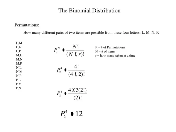
2. R - Binomial Distribution The binomial distribution model deals with finding the probability of success of an event which has only two possible outcomes in a series of experiments. For example, tossing of a coin always gives a head or a tail. The probability of finding exactly 3 heads in tossing a coin repeatedly for 10 times is estimated during the binomial distribution.

3. R has four in-built functions to generate binomial distribution. They are described below:- dbinom(x, size, prob) pbinom(x, size, prob) qbinom(p, size, prob) rbinom(n, size, prob) Following is the description of the parameters used:- x is a vector of numbers. p is a vector of probabilities. n is number of observations. size is the number of trials. prob is the probability of success of each trial.

4. dbinom() This function gives the probability density distribution at each point. # Create a sample of 50 numbers which are incremented by 1. x <- seq(0,50,by = 1) # Create the binomial distribution. y <- dbinom(x,50,0.5) # Give the chart file a name. png(file = "dbinom.png") # Plot the graph for this sample. plot(x,y) # Save the file. dev.off()

5. When we execute the above code, it produces the following result :-

6. pbinom() This function gives the cumulative probability of an event. It is a single value representing the probability. # Probability of getting 26 or less heads from a 51 tosses of a coin. x <- pbinom(26,51,0.5) print(x) When we execute the above code, it produces the following result:- 0.610116

7. qbinom() This function takes the probability value and gives a number whose cumulative value matches the probability value. # How many heads will have a probability of 0.25 will come out when a coin # is tossed 51 times. x <- qbinom(0.25,51,1/2) print(x) When we execute the above code, it produces the following result:- 23

8. rbinom() This function generates required number of random values of given probability from a given sample. # Find 8 random values from a sample of 150 with probability of 0.4. x <- rbinom(8,150,.4) print(x) When we execute the above code, it produces the following result 58 61 59 66 55 60 61 67

9. Topics for next Post R - Poisson Regression R - Time Series Analysis R - Nonlinear Least Square Stay Tuned with