Mesoscale Model Evaluation
The evaluation of high-resolution mesoscale forecasts presents unique challenges in meteorology. Traditional verification methods often fall short in addressing the complexity of forecast behavior and the realistic nature of phenomena. This presentation outlines the inadequacies of existing verification techniques, proposing innovative solutions that focus on the realistic characteristics and structures of weather patterns. We explore the importance of measuring specific performance aspects and present an "object-oriented" approach that utilizes automated techniques for characterizing and verifying forecasted and observed weather phenomena effectively.


Mesoscale Model Evaluation
E N D
Presentation Transcript
Mesoscale Model Evaluation Mike Baldwin Cooperative Institute for Mesoscale Meteorological Studies, University of Oklahoma Also affiliated with NOAA/NSSL and NOAA/NWS/SPC
NWS – forecasts on hi-res grids • What would you suggest that NWS do to verify these forecasts?
Issues in mesoscale verification • Validate natural behavior of forecasts • Realistic variability, structure of fields • Do predicted events occur with realistic frequency? • Do characteristics of phenomena mimic those found in nature? • Traditional objective verification techniques are not able to address these issues
Outline • Problems with traditional verification • Solutions: • Verify characteristics of phenomena • Verify structure/variability • Design verification systems that address value of forecasts
Traditional verification • Compare a collection of matching pairs of forecast and observed values at the same set of points in space/time • Compute various measures of accuracy: RMSE, bias, equitable threat score • A couple of numbers may represent the accuracy of millions of model grid points, thousands of cases, hundreds of meteorological events • Boiling down that much information into one or two numbers is not very meaningful
Dimensionality of verification info • Murphy (1991) and others highlight danger of simplifying complex verification information • High-dimension information = data overload • Verification information should be easy to understand • Need to find ways to measure specific aspects of performance
Quality vs. value • Scores typically measure quality, or degree in which forecasts and observations agree • Forecast value is benefit of forecast information to decision maker • Value is subjective, complex function of quality • High-quality forecast may be of low value and vice versa
OBSERVED FCST #1: smooth Forecast #1: smooth OBSERVED FCST #2: detailed
Traditional “measures-oriented” approach to verifying these forecasts
Phase/timing errors • High-amplitude, small-scale forecast and observed fields are most sensitive to timing/phase errors
Mean Squared Error (MSE) • For 1 point phase error MSE = 0.0016
Mean Squared Error (MSE) • For 1 point phase error MSE = 0.165
Mean Squared Error (MSE) • For 1 point phase error MSE = 1.19
Verify forecast “realism” • Anthes (1983) paper suggests several ways to verify “realism” • Verify characteristics of phenomena • Decompose forecast errors as function of spatial scale • Verify structure/variance spectra
Characterize the forecast and observed fields • Verify the forecast with a similar approach as a human forecaster might visualize the forecast/observed fields • Characterize features, phenomena, events, etc. found in forecast and observed fields by assigning attributes to each object • Not an unfamiliar concept: • “1050 mb high” • “category 4 hurricane” • “F-4 tornado”
Many possible ways to characterize phenomena • Shape, orientation, size, amplitude, location • Flow pattern • Subjective information (confidence, difficulty) • Physical processes in a NWP model • Verification information can be stratified using this additional information
“Object-oriented” approach to verification • Decompose fields into sets of “objects” that are identified and described by a set of attributes in an automated fashion • Using image processing techniques to locate and identify events • Produce “scores” or “metrics” based upon the similarity/dissimilarity between forecast and observed events • Could also examine the joint distribution of forecast and observed events
Characterization: How? • Identify an object Usually involves complex image processing Event #16
Characterization: How? • Assign attributes Examples: location, mean, orientation, structure Event #16: Lat=37.3N, Lon=87.8W, q=22.3, b=2.1
Automated rainfall object identification • Contiguous regions of measurable rainfall (similar to CRA; Ebert and McBride (2000))
Expand area by 15%, connect regions that are within 20km, relabel
Object characterization • Compute attributes
fcst #1 fcst #2 Verification of detailed forecasts observed RMSE = 3.4 MAE = 0.97 ETS = 0.06 • 12h forecasts of 1h precipitation valid 00Z 24 Apr 2003 RMSE = 1.7 MAE = 0.64 ETS = 0.00
fcst #1 fcst #2 Verification b = 7.8 ecc 20 = 3.6 ecc 40 = 3.1 ecc 60 = 4.5 ecc 80 = 3.6 observed • 12h forecasts of 1h precipitation valid 00Z 24 Apr 2003 b = 3.1 ecc 20 = 2.6 ecc 40 = 2.0 ecc 60 = 2.1 ecc 80 = 2.8 b = 1.6 ecc 20 = 10.7 ecc 40 = 7.5 ecc 60 = 4.3 ecc 80 = 2.8
Example of scores produced by this approach • fi = (ai, bi, ci, …, xi, yi)t • ok= (ak, bk, ck, …, xk, yk)t • di,k(fi,ok) = (fi-ok)t A (fi-ok) (Generalized Euclidean distance, measure of dissimilarity) where A is a matrix, different attributes would probably have different weights • ci,k(fi,ok) = cov(fi,ok) (measure of similarity)
Ebert and McBride (2000) • Contiguous Rain Areas • Separate errors into amplitude, displacement, shape components
Contour error map (CEM) method • Case et al (2003) • Phenomena of interest – Florida sea breeze • Object identification – sea breeze transition time • Contour map of transition time errors • Distributions of timing errors • Verify post-sea breeze winds
Nachamkin (2004) Identify events of interest in the forecasts Collect coordinated samples Compare forecast PDF to observed PDF Repeat process for observed events Compositing
Decompose errors as a function of scale • Bettge and Baumhefner (1980) used band-pass filters to analyze errors at different scales • Briggs and Levine (1997) used wavelet analysis of forecast errors
Verify structure • Fourier energy spectra • Take Fourier transform, multiply by complex conjugate – E(k) • Display on log-log plot • Natural phenomena often show “power-law” regimes • Noise (uncorrelated) results in flat spectrum
Fourier spectra • Slope of spectrum indicates degree of structure in the data
Larger absolute values of slope correspond with less structure slope = -1 noise slope = -1.5 slope = -3
Multiscale statistical properties (Harris et al 2001) • Fourier energy spectrum • Generalized structure function: spatial correlation • Moment-scale analysis: intermittency of a field, sparseness of sharp intensities • Looking for “power law”, much like in atmospheric turbulence (–5/3 slope) FIG. 3. Isotropic spatial Fourier power spectral density (PSD) for forecast RLW (qr; dotted line) and radar-observed qr (solid line). Comparison of the spectra shows reasonable agreement at scales larger than 15 km. For scales smaller than 15 km, the forecast shows a rapid falloff in variability in comparison with the radar. The estimated spectral slope with fit uncertainty is = 3.0 ± 0.1
Example Obs_4 Eta_12 Eta_8 log[E(k)] log[wavenumber] 3-6h forecasts from 04 June 2002 1200 UTC WRF_22 WRF_10 KF_22
Comparing forecasts that contain different degrees of structure Obs=black Detailed = blue Smooth = green MSE detailed = 1.57 MSE smooth = 1.43
Common resolved scales vs. unresolved • Filter other forecasts to have same structure • MSE “detailed” = 1.32 • MSE smooth = 1.43
Lack of detail in analyses • Methods discussed assume realistic analysis of observations • Problems: Relatively sparse observations • Operational data assimilation systems • Smooth first guess fields from model forecasts • Smooth error covariance matrix • Smooth analysis fields result
True mesoscale analyses • Determine what scales are resolved • Mesoscale data assimilation • Frequent updates • All available observations • Hi-res NWP provides first guess • Ensemble Kalman filter • Tustison et al. (2002) scale-recursive filtering takes advantage of natural “scaling”
Design verification systems that address forecast value • Value measures the benefits of forecast information to users • Determine what aspects of forecast users are most sensitive to • If possible, find out users “cost/loss” situation • Are missed events or false alarms more costly?
Issues • How to distill the huge amount of verification information into meaningful “nuggets” that can be used effectively? • How to elevate verification from an annoyance to an integral part of the forecast process? • What happens when conflicting information from different verification approaches is obtained?
Summary • Problems with traditional verification techniques when used with forecasts/observations with structure • Verify realism • Issues of scale • Work with forecasters/users to determine most important aspects of forecast information
References • Good books • Papers mentioned in this presentation • Beth Ebert’s website
Scores based on similarity/dissimilarity matrices • D = [di,j] euclidean distance matrix • C = [ci,j] covariance matrix • Scores could be: tr[D] = trace of matrix, for euclidean distance this equates to S (fi – oi)2 ~ RMSE det[D] = determinant of matrix, a measure of the magnitude of a matrix