Download
1 / 48
480 likes | 589 Views
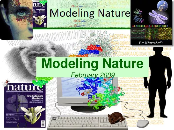
Modeling Nature February 2009. Modeling Nature. LECTURE 2: Predator-prey models * and more general information …. Task descriptions and required readings. Each lecture has two associated tasks ( a , b ) The task descriptions can be found on ELEUM

E N D
Modeling Nature LECTURE 2: Predator-prey models * and more general information …
Task descriptions and required readings • Each lecture has two associated tasks (a, b) • The task descriptions can be found on ELEUM • Each task has a number of required readings on the ELEUM website • Additional readings and Web pointers are also available (not mandatory, but useful)
Task Descriptions • Updated task descriptions of are made available through ELEUM on a weekly basis • Note that the task descriptions in the course manual (syllabus) become over-ruled by these new descriptions !!!
Student research project A TEAM consists of 2 to 3 students A 2-3 PAGE PROPOSAL is submitted ultimately on Monday 2 March to the tutor of the team’s TG. PRESENTATION: +/-10 minutes each presentation in the week of 23 March in the TGs. REPORT: a short paper (2500 words) on the subject. THE GRADE is for the TEAM and thus for all students in the TEAM. It consists of 50% for the report and 50% for the presentation.
Complete time table • 02/2 - Lecture 1 : Models, Growth & Decay • 09/2 - Lecture 2 : Predator-Prey Systems • 16/2 - Lecture 3 : Network Models • 02/3 - Lecture 4 : Chaos and Fractals; first draft report and presentation – feedback from tutors • 09/3 - Lecture 5 : Percolation and Phase Transitions • 16/3 - Lecture 6 : Self-Organization and Collective Phenomena • 23/3 - Week 7 : Student presentations on chosen topic; report • 30/3 - Week 8 : Final exam
Final mark of the course The final mark of the course consists of 40% of the project and 60% of the written exam. Only students with sufficient attendance may attend the exam and present his/her project, when only 1 TG lacks for a valid pass, the student receives an additional task, otherwise the students fails the course.
General Information More questions? Ask after the Lecture or your personal tutor
Lecture 2: PREDATOR-PREY SYSTEMS
Overview • From one to two equations • Volterra’s model of predator-prey (PP) systems • Why are PP models useful? • Examples from nature • Relation to future tasks
Recall the Logistic Model • Pn is the fraction of the maximum population size 1 • is a parameter that describes the strength of the coupling Large P slows down P Logistic model a.k.a. the Verhulst model
Interacting quantities • The logistic model describes the dynamics (change) of a single quantity interacting with itself • We now move to models describing two (or more) interacting quantities
Fish statistics • Vito Volterra (1860-1940): a famous Italian mathematician • Father of Humberto D'Ancona, a biologist studying the populations of various species of fish in the Adriatic Sea • The numbers of species sold on the fish markets of three ports: Fiume, Trieste, and Venice.
predator prey Volterra’s model • Two (simplifying) assumptions • The predator species is totally dependent on the prey species as its only food supply • The prey species has an unlimited food supply and no threat to its growth other than the specific predator
predator prey Lotka–Volterra equation : The Lotka–Volterra equations are a pair of equations used to describe the dynamics of biological systems in which two species interact, one a predator and one its prey. They were proposed independently by Alfred J. Lotka in 1925 and Vito Volterra in 1926.
Two species species #1: population size: x species #2: population size: y Lotka–Volterra equation :
Lotka–Volterra equation : Remember Verhulst-equation: Predator (x) and prey (y) model: xn+1= xn(α – βyn) : yis the limitation forx yn+1= yn(γ – δxn) : xis the limitation fory
Equivalent formulation: rate of change: dx/dt = in/de-crease per unit time (e.g. 2000 hares per year) Lotka–Volterra equation :
Behaviour of the Volterra’s model Oscillatory behaviour Limit cycle
Effect of changing the parameters (1) Behaviour is qualitatively the same. Only the amplitude changes.
Effect of changing the parameters (2) Behaviour is qualitatively different. A fixed point instead of a limit cycle.
Predator-prey interaction in vivo Huffaker (1958) reared two species of mites to demonstrate coupled oscillations of predator and prey densities in the laboratory. He used Typhlodromus occidentalis as the predator and the six-spotted mite (Eotetranychus sexmaculatus) as the prey
http://www.xjtek.com/models/?archive=ecosystem_dynamics/predator_prey/model.jar,xjanylogic6engine.jar&root=predator_prey.Simulation$Applet&width=800&height=650&version=6http://www.xjtek.com/models/?archive=ecosystem_dynamics/predator_prey/model.jar,xjanylogic6engine.jar&root=predator_prey.Simulation$Applet&width=800&height=650&version=6 Online simulation of PP model
Exponential growth Limited growth Exponential decay Oscillation Why are PP models useful? • They model the simplest interaction among two systems and describe natural patterns • Repetitive growth-decay patterns, e.g., • World population growth • Diseases • … time
Lynx and hares Very few "pure" predator-prey interactions have been observed in nature, but there is a classical set of data on a pair of interacting populations that come close: the Canadian lynx and snowshoe hare pelt-trading records of the Hudson Bay Company over almost a century.
The Hudson Bay data give us a reasonable picture of predator-prey interaction over an extended period of time. The dominant feature of this picture is the oscillating behavior of both populations
what is the period of oscillation of the lynx population? • what is the period of oscillation of the hare population? • do the peaks of the predator population match or slightly precede or slightly lag those of the prey population?
“equilibrium” states • Complex systems are assumed to converge towards an equilibrium state.Equilibrium state: two (or more) opposite processes take place at equal rates unstable stable
More complicated interactions [1] • Clinton established the Giant Sequoia National Monument to protect the forest from culling, logging and clearing. • But many believe that Clinton’s measures added fuel to the fires. • Tree-thinning is required to prevent large fires. • Fires are required to clear land and to promote new growth.
Fire is dangerous when caused by surrounding bushes Fire is needed to clean area and to open the seeds of the Sequoia Predator versus Prey? • Fire acts as “prey” because it is needed for growth • Fire acts as “predator” because it may set the tree on fire • Tree acts as “prey” for the predator • If trees die out, the predator dies out too
More complicated interactions [2] Predators, Preys and Hurricanes
More complicated interactions [3] Biodiversity “Human alteration of the global environment has triggered the sixth major extinction event in the history of life and caused widespread changes in the global distribution of organisms. These changes in biodiversity alter ecosystem processes and change the resilience of ecosystems to environmental change. This has profound consequences for services that humans derive from ecosystems. The large ecological and societal consequences of changing biodiversity should be minimized to preserve options for future solutions to global environmental problems.” F. Stuart Chapin III et al. (2000)
Consequences of reduced biodiversity "...decreasing biodiversity will tend to increase the overall mean interaction strength, on average, and thus increase the probability that ecosystems undergo destabilizing dynamics and collapses." Kevin Shear McCann (2000)