Download
1 / 25
250 likes | 320 Views
These notes discuss high-latitude ionosphere's electrodynamic characteristics, E-field signatures, space observations, and current sheet approximations for interpreting satellite encounters.

E N D
Aurorae and High-Latitude Electrodynamics The Physics of Space Plasmas William J. Burke24 October 2012 University of Massachusetts, Lowell
Aurorae and High-Latitude Electrodynamics Lecture 6 • These notes deal primarily with the electrodynamic characteristics of the high-latitude ionosphere. • We briefly review the expected signatures of electric potential and field-aligned current distributions during southward IMF BZ intervals. • Examine ground- and space-based observations near the dayside cusp, emphasizing responsiveness to changes in IMF orientations. • Examine in detail E and B variations associated with the infinite current sheet approximation and apply them to a interpreting acase frequently encountered by satellites near the open-closed boundary in the evening MLT sector.
Aurorae and High-Latitude Electrodynamics Iijima and Potemra, JGR, 1978 Heppner and Maynard, JGR, 1987 • Pattern-recognition, steady-state guides that should not be taken too literally • No E-fields represented at magnetic latitudes < 60.They are measureable with reversed polarities during main and early recovery of magnetic storms. • There exist extended regions in which E 0 quasi neutrality preserved. • How do we join them?
Aurorae and High-Latitude Electrodynamics • Schematic for interpreting EX and • dBY measurements from a s/c in polar-orbit along dawn dusk meridian. • Satellite-based coordinates • X positive along s/c trajectory • Y positive in anti-sunward direction • Z positive toward nadir j||1 j||1 j||2 j||2 dBY dBY dBY dBY dBY dBY EX dBY j||2 j||2 j||1 j||1
Aurorae and High-Latitude Electrodynamics Heppner-Maynard, JGR, 1987 Northern Hemisphere: BY > 0, BZ < 0 Northern Hemisphere : BY < 0, BZ < 0 Model BC Model DE Southern Hemisphere: BY < 0, BZ < 0 Southern Hemisphere: BY > 0, BZ < 0
Aurorae and High-Latitude Electrodynamics Dayside FAC System Erlandson et al., JGR, 1988 Dayside Precipitation Pattern Newell and Meng, GRL, 1992 Heppner - Maynard Convection Patterns (JGR, 1987)
Aurorae and High-Latitude Electrodynamics Nopper and Carovillano, GRL 699, 1978 Region 1 = 106 A Region 2 = 3105 A Region 1 = 106 A Region 2 = 0 A Wolf, R. A., Effects of Ionospheric Conductivity on Convective Flow of Plasma in the Magnetosphere, JGR, 75, 4677, 1970.
Aurorae and Dayside Cusp Sandholt et al. , JGR 1998
Aurorae and Dayside Cusp Sandholt et al., JGR 1993
Aurorae and Dayside Cusp 5577 Å emissions monitored by all-sky imager at Ny Ålesund after 09:00 UT on 19 December 2001. The colored lines are placed at constant positions as guide to the eye for discerning optical changes.
Aurorae and High-Latitude Electrodynamics Inverted Vs Polar Rain F15 / F13 crossed local noon MLT at ~ 09:22 an 09:36 UT
Aurorae and High-Latitude Electrodynamics Top right: 6300 Å emissions mapped to 220 km. All 5577 Å emissions mapped to an altitude of 190 km. Middle traces indicate that 5577 Å variations are responses to changes in the IMF clock angle.
Aurorae and High-Latitude Electrodynamics Fridman, M., and J. Lemaire, JGR, 664, 1980. Kan and Lee, JGR, 788, 1979.
Discrete Aurorae: Current –Voltage Relation • Consider a trapped electron population with an isotropic, Maxwellian distribution function whose mean thermal energy = Eth • Assume that there is a field-aligned potential drop V|| that begins at a height where the magnetic field strength is BV||. • Knight (PSS, 741, 1973) showed that j||carried by precipitating electrons is given by the top equation, where Bi is the magnetic field strength at the ionosphere. Lyons, JGR, 17, 1980 j|| - V|| Relationship
Infinite Current Sheet Approximation Normal Incidence Oblique Incidence
Infinite Current Sheet Approximation If ( = 0), then Y Normal Incidence j|| = (1/ 0) [YBZ] = (1/ Vsat 0) [t BZ] Vsat 7.5 km/s 1 A/m2 9.4 nT/s J|| = ∫ j|| dY J|| = (1/ 0) [ BZ]1 A/m BZ = 1256 nT In DMSP-centered coordinates: j|| = Y [PEY - HEZ] = (1/ 0) [YBZ] Oblique Incidence Y [ BZ - 0 ( PEY - HEZ)] = 0 Where BZ andEY vary in the same way P ≈ (1/ 0) [ BZ / EY].
Infinite Current Sheet Approximation Normal Incidence Oblique Incidence
Infinite Current Sheet Approximation Let Y (VS Cos )-1 d/dt, and assume: H = P then Normal Incidence Oblique Incidence In regions where EY’ and BZ’ are highly correlated
Infinite Current Sheet Approximation and Normal Incidence Since in = 4.2 ×10⁻¹⁰ nn and Oblique Incidence weak transverse gradients in are expected. Solar EUV Electron Precipitation Robinson et al., JGR, 92, 2565, 1987. E0 = mean thermal energy in keV I = energy flux in ergs/cm2-s
Infinite Current Sheet Approximation VY > 0 eastward flowSpike always occurred at the poleward boundary of auroral electron precipitation Dynamics Explorer 2 saw similar features: - Double probe - Triaxial fluxgate magnetometer - Drift meter and RPA Burke et al., ,J. Geophys. Res., 99, 2489, 1994.
Infinite Current Sheet Approximation • EX peak coincided with auroral electron boundary, but not with the BZ peak P,H gradients. • Convection reversal inside of R1 FAC • BZ decreased by 220 nT between 07:38 and 07:39 UT j|| = 0.44 A/m2 • EX and BZ variations in R0 consistent with P 2 mho • Auroral electrons underwent field-aligned accelerations of ~ 7 keV • BX and BZ variations in R1 indicate an attack angle of ~ 18 • From RPA: Etang 10 mV/m R1 R0 R2
Infinite Current Sheet Approximation • Assumed P H and set X0 at 07:37 UT • X = X0 + Vsat t Bmax = 275 nT • Integrated numerically