Download
1 / 25
250 likes | 358 Views
CS 290H Administrivia: April 9, 2008. Homework 2 due next Wednesday (see web site). Reading in Davis: Sections 4.8 and 4.11 (left-looking Cholesky) Sections 6.1 and 6.2 (left-looking LU) A few copies of Davis are still available at a discount from Roxanne in HFH 5102. 1. 2. 3. 4. 5.

E N D
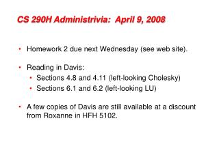
CS 290H Administrivia: April 9, 2008 • Homework 2 due next Wednesday (see web site). • Reading in Davis: • Sections 4.8 and 4.11 (left-looking Cholesky) • Sections 6.1 and 6.2 (left-looking LU) • A few copies of Davis are still available at a discount from Roxanne in HFH 5102.
1 2 3 4 5 = 1 3 5 2 4 Sparse Triangular Solve L x b G(LT) • Symbolic: • Predict structure of x by depth-first search from nonzeros of b • Numeric: • Compute values of x in topological order Time = O(flops)
dfs in G(LT) to predict nonzeros of x;x(1:n) = b(1:n); // copy b into a SPA for xfor i = nonzero indices of x in topological order x(i) = x(i) / L(i, i); x(i+1:n) = x(i+1:n) – L(i+1:n, i) * x(i); end;store SPA into x in CSC form & reset the SPA; Sparse-sparse triangular solve: x = L \ b • Depth-first search calls “visit” once per flop • Runs in O(flops) time even if it’s less than nnz(L) or n … • Except for one-time O(n) SPA setup
Nonsymmetric Ax = b: Gaussian elimination (without pivoting) • Factor A = LU • Solve Ly = b for y • Solve Ux = y for x • Variations: • Pivoting for numerical stability: PA=LU • Cholesky for symmetric positive definite A: A = LLT • Permuting A to make the factors sparser = x
for column j = 1 to n do solve scale:lj = lj / ujj j U L A ( ) L 0L I ( ) ujlj L = aj for uj, lj Left-looking Column LU Factorization • Column j of A becomes column j of L and U
L = speye(n);for column j = 1 : ndfs in G(LT) to predict nonzeros of x; x(1:n) = A(1:n, j); // x is a SPA for i = nonzero indices of x in topological order x(i) = x(i) / L(i, i); x(i+1:n) = x(i+1:n) – L(i+1:n, i) * x(i); U(1:j, j) = x(1:j); L(j+1:n, j) = x(j+1:n);cdiv: L(j+1:n, j) = L(j+1:n, j) / U(j, j); Left-looking sparse LU without pivoting (simple)
GPLU Algorithm [1988] • Left-looking column-by-column factorization • Depth-first search to predict structure of each column • Partial pivoting +: Symbolic analysis cost proportional to flops -: Big constant factor – symbolic cost still dominates => Prune symbolic representation
j k r r = fill Symmetric pruning:Set Lsr=0 if LjrUrj 0 Justification:Ask will still fill in j = pruned = nonzero s Symmetric Pruning [Eisenstat, Liu] Idea: Depth-first search in a sparser graph with the same path structure • Use (just-finished) column j of L to prune earlier columns • No column is pruned more than once • The pruned graph is the elimination tree if A is symmetric
L = speye(n); S = empty n-vertex graph;for column j = 1 : ndfs in S to predict nonzeros of x; x(1:n) = A(1:n, j); // x is a SPA for i = nonzero indices of x in topological order x(i) = x(i) / L(i, i); x(i+1:n) = x(i+1:n) – L(i+1:n, i) * x(i); U(1:j, j) = x(1:j); L(j+1:n, j) = x(j+1:n); cdiv: L(j+1:n, j) = L(j+1:n, j) / U(j, j);update S: add edges (j, i) for nonzero L(i, j);prune S using L(j+1:n,j); Left-looking sparse LU without pivoting (pruned)
Nonsymmetric Ax = b: Gaussian elimination with partial pivoting At step j, swap the unused row with largest diagonal element into the pivot position. • Factor PA = LU • Solve Ly = Pb for y • Solve Ux = y for x P = x
for column j = 1 to n do solve pivot: swap ujj and an elt of lj scale:lj = lj / ujj j U L A ( ) L 0L I ( ) ujlj L = aj for uj, lj Left-looking Column LU Factorization • Column j of A becomes column j of L and U
L = speye(n); S = empty n-vertex graph;for column j = 1 : ndfs in S to predict nonzeros of x; x(1:n) = A(1:n, j); // x is a SPA for i = nonzero indices of x in topological order x(i) = x(i) / L(i, i); x(i+1:n) = x(i+1:n) – L(i+1:n, i) * x(i); U(1:j, j) = x(1:j); L(j+1:n, j) = x(j+1:n); pivot: swap U(j, j) and an element of L(:, j);cdiv: L(j+1:n, j) = L(j+1:n, j) / U(j, j);update S: add edges (j, i) for nonzero L(i, j);prune S using L(j+1:n,j); Left-looking sparse LU with partial pivoting (pruned)
GPMOD Algorithm [Eisenstat, Liu 1993] • Left-looking column-by-column factorization • Depth-first search to predict structure of each column • Symmetric pruning to reduce symbolic cost • Partial pivoting +: Much cheaper symbolic factorization than GPLU (~4x) -: Indirect addressing for each flop (sparse vector kernel) -: Poor reuse of data in cache (BLAS-1 kernel) => Supernodes
{ Symmetric supernodes for Cholesky [Davis section 4.8] • Supernode = group of adjacent columns of L with same nonzero structure • Related to clique structureof filled graph G+(A) • Supernode-column update: k sparse vector ops become 1 dense triangular solve + 1 dense matrix * vector + 1 sparse vector add • Sparse BLAS 1 => Dense BLAS 2 • Only need row numbers for first column in each supernode • For model problem, integer storage for L is O(n) not O(n log n)
1 1 2 2 3 3 4 4 5 5 6 6 7 7 8 8 9 9 10 10 Factors L+U Nonsymmetric Supernodes Original matrix A
for each panel do Symbolic factorization:which supernodes update the panel; Supernode-panel update:for each updating supernode do for each panel column dosupernode-column update; Factorization within panel:use supernode-column algorithm +: “BLAS-2.5” replaces BLAS-1 -: Very big supernodes don’t fit in cache => 2D blocking of supernode-column updates j j+w-1 } } supernode panel Supernode-Panel Updates
Sequential SuperLU [1999] • Depth-first search, symmetric pruning • Supernode-panel updates • 1D or 2D blocking chosen per supernode • Blocking parameters can be tuned to cache architecture • Condition estimation, iterative refinement, componentwise error bounds
SuperLU: Relative Performance • Speedup over GPLU column-column • 22 matrices: Order 765 to 76480; GP factor time 0.4 sec to 1.7 hr • SGI R8000 (1995)
Sparse Cholesky factorization to solve Ax = b • Preorder: replace A by PAPT and b by Pb • Independent of numerics • Symbolic Factorization: build static data structure • Elimination tree • Nonzero counts • Supernodes • Nonzero structure of L • Numeric Factorization: A = LLT • Static data structure • Supernodes use BLAS3 to reduce memory traffic • Triangular Solves: solve Ly = b, then LTx = y
for j = 1 : n for k = 1 : j -1 % cmod(j,k) for i = j : n A(i, j) = A(i, j) – A(i, k)*A(j, k); end; end; % cdiv(j) A(j, j) = sqrt(A(j, j)); for i = j+1 : n A(i, j) = A(i, j) / A(j, j); end; end; j LT L A L Column Cholesky Factorization • Column j of A becomes column j of L
for j = 1 : n L(j:n, j) = A(j:n, j); for k < j with L(j, k) nonzero % sparse cmod(j,k) L(j:n, j) = L(j:n, j) – L(j, k) * L(j:n, k); end; % sparse cdiv(j) L(j, j) = sqrt(L(j, j)); L(j+1:n, j) = L(j+1:n, j) / L(j, j); end; j LT L A L Sparse Column Cholesky Factorization • Column j of A becomes column j of L
3 7 1 3 7 1 6 8 6 8 4 10 4 10 9 2 9 2 5 5 Graphs and Sparse Matrices: Cholesky factorization Fill:new nonzeros in factor Symmetric Gaussian elimination: for j = 1 to n add edges between j’s higher-numbered neighbors G+(A)[chordal] G(A)
Path lemma (Davis Theorem 4.1) Let G = G(A) be the graph of a symmetric, positive definite matrix, with vertices 1, 2, …, n, and let G+ = G+(A)be the filled graph. Then (v, w) is an edge of G+if and only if G contains a path from v to w of the form (v, x1, x2, …, xk, w) with xi < min(v, w) for each i. (This includes the possibility k = 0, in which case (v, w) is an edge of G and therefore of G+.)
3 7 1 6 8 10 4 10 9 5 4 8 9 2 2 5 7 3 6 1 Elimination Tree G+(A) T(A) Cholesky factor • T(A) : parent(j) = min { i > j : (i, j) inG+(A) } • parent(col j) = first nonzero row below diagonal in L • T describes dependencies among columns of factor • Can compute G+(A) easily from T • Can compute T from G(A) in almost linear time
Facts about elimination trees • If G(A) is connected, then T(A) is connected (it’s a tree, not a forest). • If A(i, j) is nonzero and i > j, then i is an ancestor of j in T(A). • If L(i, j) is nonzero, then i is an ancestor of j in T(A). • T(A) is a depth-first spanning tree of G+(A). • T(A) is the transitive reduction of the directed graph G(LT).