Download

1 / 52
520 likes | 670 Views
EE4800 CMOS Digital IC Design & Analysis . Lecture 8 Spice Simulation Zhuo Feng. Outline. Introduction to SPICE DC Analysis Transient Analysis Subcircuits Optimization Power Measurement Logical Effort Characterization. Introduction to SPICE.

E N D
EE4800 CMOS Digital IC Design & Analysis Lecture 8 Spice Simulation Zhuo Feng
Outline • Introduction to SPICE • DC Analysis • Transient Analysis • Subcircuits • Optimization • Power Measurement • Logical Effort Characterization
Introduction to SPICE • Simulation Program with Integrated Circuit Emphasis • Developed in 1970’s at Berkeley • Many commercial versions are available • HSPICE is a robust industry standard • Has many enhancements that we will use • Written in FORTRAN for punch-card machines • Circuits elements are called cards • Complete description is called a SPICE deck
Writing Spice Decks • Writing a SPICE deck is like writing a good program • Plan: sketch schematic on paper or in editor • Modify existing decks whenever possible • Code: strive for clarity • Start with name, email, date, purpose • Generously comment • Test: • Predict what results should be • Compare with actual • Garbage In, Garbage Out!
Example: RC Circuit * rc.sp * David_Harris@hmc.edu 2/2/03 * Find the response of RC circuit to rising input *------------------------------------------------ * Parameters and models *------------------------------------------------ .option post *------------------------------------------------ * Simulation netlist *------------------------------------------------ Vin in gnd pwl 0ps 0 100ps 0 150ps 1.8 800ps 1.8 R1 in out 2k C1 out gnd 100f *------------------------------------------------ * Stimulus *------------------------------------------------ .tran 20ps 800ps .plot v(in) v(out) .end
Result (Textual) legend: a: v(in) b: v(out) time v(in) (ab ) 0. 500.0000m 1.0000 1.5000 2.0000 + + + + + 0. 0. -2------+------+------+------+------+------+------+------+- 20.0000p 0. 2 + + + + + + + + 40.0000p 0. 2 + + + + + + + + 60.0000p 0. 2 + + + + + + + + 80.0000p 0. 2 + + + + + + + + 100.0000p 0. 2 + + + + + + + + 120.0000p 720.000m +b + + a+ + + + + + 140.0000p 1.440 + b + + + + + a + + + 160.0000p 1.800 + +b + + + + + +a + 180.0000p 1.800 + + b + + + + + +a + 200.0000p 1.800 -+------+------+b-----+------+------+------+------+a-----+- 220.0000p 1.800 + + + b + + + + +a + 240.0000p 1.800 + + + +b + + + +a + 260.0000p 1.800 + + + + b + + + +a + 280.0000p 1.800 + + + + b+ + + +a + 300.0000p 1.800 + + + + +b + + +a + 320.0000p 1.800 + + + + + b + + +a + 340.0000p 1.800 + + + + + b + + +a + 360.0000p 1.800 + + + + + b + +a + 380.0000p 1.800 + + + + + +b + +a + 400.0000p 1.800 -+------+------+------+------+------+--b---+------+a-----+- 420.0000p 1.800 + + + + + + b + +a + 440.0000p 1.800 + + + + + + b + +a + 460.0000p 1.800 + + + + + + b+ +a + 480.0000p 1.800 + + + + + + b +a + 500.0000p 1.800 + + + + + + +b +a + 520.0000p 1.800 + + + + + + +b +a + 540.0000p 1.800 + + + + + + + b +a + 560.0000p 1.800 + + + + + + + b +a + 580.0000p 1.800 + + + + + + + b +a + 600.0000p 1.800 -+------+------+------+------+------+------+---b--+a-----+- 620.0000p 1.800 + + + + + + + b +a + 640.0000p 1.800 + + + + + + + b +a + 660.0000p 1.800 + + + + + + + b +a + 680.0000p 1.800 + + + + + + + b +a + 700.0000p 1.800 + + + + + + + b+a + 720.0000p 1.800 + + + + + + + b+a + 740.0000p 1.800 + + + + + + + b+a + 760.0000p 1.800 + + + + + + + b+a + 780.0000p 1.800 + + + + + + + ba + 800.0000p 1.800 -+------+------+------+------+------+------+------ba-----+- + + + + +
Sources • DC Source Vdd vdd gnd 2.5 • Piecewise Linear Source Vin in gnd pwl 0ps 0 100ps 0 150ps 1.8 800ps 1.8 • Pulsed Source Vck clk gnd PULSE 0 1.8 0ps 100ps 100ps 300ps 800ps
Letter Element R Resistor C Capacitor L Inductor K Mutual Inductor V Independent voltage source I Independent current source M MOSFET D Diode Q Bipolar transistor W Lossy transmission line X Subcircuit E Voltage-controlled voltage source G Voltage-controlled current source H Current-controlled voltage source F Current-controlled current source SPICE Elements
Units Ex: 100 femptofarad capacitor = 100fF, 100f, 100e-15
DC Analysis * mosiv.sp *------------------------------------------------ * Parameters and models *------------------------------------------------ .include '../models/tsmc180/models.sp' .temp 70 .option post *------------------------------------------------ * Simulation netlist *------------------------------------------------ *nmos Vgs g gnd 0 Vds d gnd 0 M1 d g gnd gnd NMOS W=0.36u L=0.18u *------------------------------------------------ * Stimulus *------------------------------------------------ .dc Vds 0 1.8 0.05 SWEEP Vgs 0 1.8 0.3 .end
I-V Characteristics • NMOS I-V • Vgs dependence • Saturation
MOSFET Elements M element for MOSFET Mname drain gate source body type + W=<width> L=<length> + AS=<area source> AD = <area drain> + PS=<perimeter source> PD=<perimeter drain>
Transient Analysis * inv.sp * Parameters and models *------------------------------------------------ .param SUPPLY=1.8 .option scale=90n .include '../models/tsmc180/models.sp' .temp 70 .option post * Simulation netlist *------------------------------------------------ Vdd vdd gnd 'SUPPLY' Vin a gnd PULSE 0 'SUPPLY' 50ps 0ps 0ps 100ps 200ps M1 y a gnd gnd NMOS W=4 L=2 + AS=20 PS=18 AD=20 PD=18 M2 y a vdd vdd PMOS W=8 L=2 + AS=40 PS=26 AD=40 PD=26 * Stimulus *------------------------------------------------ .tran 1ps 200ps .end
Transient Results • Unloaded inverter • Overshoot • Very fast edges
Subcircuits • Declare common elements as subcircuits • Ex: Fanout-of-4 Inverter Delay • Reuse inv • Shaping • Loading .subckt inv a y N=4 P=8 M1 y a gnd gnd NMOS W='N' L=2 + AS='N*5' PS='2*N+10' AD='N*5' PD='2*N+10' M2 y a vdd vdd PMOS W='P' L=2 + AS='P*5' PS='2*P+10' AD='P*5' PD='2*P+10' .ends
FO4 Inverter Delay * fo4.sp * Parameters and models *---------------------------------------------------------------------- .param SUPPLY=1.8 .param H=4 .option scale=90n .include '../models/tsmc180/models.sp' .temp 70 .option post * Subcircuits *---------------------------------------------------------------------- .global vdd gnd .include '../lib/inv.sp' * Simulation netlist *---------------------------------------------------------------------- Vdd vdd gnd 'SUPPLY' Vin a gnd PULSE 0 'SUPPLY' 0ps 100ps 100ps 500ps 1000ps X1 a b inv * shape input waveform X2 b c inv M='H' * reshape input waveform
FO4 Inverter Delay Cont. X3 c d inv M='H**2' * device under test X4 d e inv M='H**3' * load x5 e f inv M='H**4' * load on load * Stimulus *---------------------------------------------------------------------- .tran 1ps 1000ps .measure tpdr * rising prop delay + TRIG v(c) VAL='SUPPLY/2' FALL=1 + TARG v(d) VAL='SUPPLY/2' RISE=1 .measure tpdf * falling prop delay + TRIG v(c) VAL='SUPPLY/2' RISE=1 + TARG v(d) VAL='SUPPLY/2' FALL=1 .measure tpd param='(tpdr+tpdf)/2' * average prop delay .measure trise * rise time + TRIG v(d) VAL='0.2*SUPPLY' RISE=1 + TARG v(d) VAL='0.8*SUPPLY' RISE=1 .measure tfall * fall time + TRIG v(d) VAL='0.8*SUPPLY' FALL=1 + TARG v(d) VAL='0.2*SUPPLY' FALL=1 .end
Optimization • HSPICE can automatically adjust parameters • Seek value that optimizes some measurement • Example: Best P/N ratio • We’ve assumed 2:1 gives equal rise/fall delays • But we see rise is actually slower than fall • What P/N ratio gives equal delays? • Strategies • (1) run a bunch of sims with different P size • (2) let HSPICE optimizer do it for us
P/N Optimization * fo4opt.sp * Parameters and models *---------------------------------------------------------------------- .param SUPPLY=1.8 .option scale=90n .include '../models/tsmc180/models.sp' .temp 70 .option post * Subcircuits *---------------------------------------------------------------------- .global vdd gnd .include '../lib/inv.sp' * Simulation netlist *---------------------------------------------------------------------- Vdd vdd gnd 'SUPPLY' Vin a gnd PULSE 0 'SUPPLY' 0ps 100ps 100ps 500ps 1000ps X1 a b inv P='P1' * shape input waveform X2 b c inv P='P1' M=4 * reshape input X3 c d inv P='P1' M=16 * device under test
P/N Optimization X4 d e inv P='P1' M=64 * load X5 e f inv P='P1' M=256 * load on load * Optimization setup *---------------------------------------------------------------------- .param P1=optrange(8,4,16) * search from 4 to 16, guess 8 .model optmod opt itropt=30 * maximum of 30 iterations .measure bestratio param='P1/4' * compute best P/N ratio * Stimulus *---------------------------------------------------------------------- .tran 1ps 1000ps SWEEP OPTIMIZE=optrange RESULTS=diff MODEL=optmod .measure tpdr * rising propagation delay + TRIG v(c) VAL='SUPPLY/2' FALL=1 + TARG v(d) VAL='SUPPLY/2' RISE=1 .measure tpdf * falling propagation delay + TRIG v(c) VAL='SUPPLY/2' RISE=1 + TARG v(d) VAL='SUPPLY/2' FALL=1 .measure tpd param='(tpdr+tpdf)/2' goal=0 * average prop delay .measure diff param='tpdr-tpdf' goal = 0 * diff between delays .end
P/N Results • P/N ratio for equal delay is 3.6:1 • tpd = tpdr = tpdf = 84 ps (slower than 2:1 ratio) • Big pMOS transistors waste power too • Seldom design for exactly equal delays • What ratio gives lowest average delay? .tran 1ps 1000ps SWEEP OPTIMIZE=optrange RESULTS=tpd MODEL=optmod • P/N ratio of 1.4:1 • tpdr = 87 ps, tpdf = 59 ps, tpd = 73 ps
Power Measurement • HSPICE can measure power • Instantaneous P(t) • Or average P over some interval .print P(vdd) .measure pwr AVG P(vdd) FROM=0ns TO=10ns • Power in single gate • Connect to separate VDD supply • Be careful about input power
Logical Effort • Logical effort can be measured from simulation • As with FO4 inverter, shape input, load output
Logical Effort Plots • Plot tpd vs. h • Normalize by t • y-intercept is parasitic delay • Slope is logical effort • Delay fits straight line very well in any process as long as input slope is consistent t= 15 ps
Logical Effort Data • For NAND gates in TSMC 180 nm process: • Notes: • Parasitic delay is greater for outer input • Average logical effort is better than estimated
l l l l • SPICE overview • N equations in terms of N unknown Node voltages • More generally using modified nodal analysis
Time Domain Equations at node 1: uIf we do this for all N nodes: N dimensional vector of unknown node voltages vector of independent sources nonlinear operator
Closed form solution is not possible for arbitrary order of differential equations • We must approximate the solution of: • This is facilitated in SPICE via numerical solutions
Basic circuit analyses • (Nonlinear) DC analysis • Finds the DC operating point of the circuit • Solves a set of nonlinear algebraic eqns • AC analysis • Performs frequency-domain small-signal analysis • Require a preceding DC analysis • Solves a set of complex linear eqns • (Nonlinear) transient analysis • Computes the time-domain circuit transient response • Solves a set of nonlinear different eqns • Converts to a set nonlinear algebraic of eqns using numerical integration
SPICE offers practical techniques to solve circuit problems in time & freq. domains • Interface to device models • Transistors, diodes, nonlinear caps etc • Sparse linear solver • Nonlinear solver – Newton-Raphson method • Numerical integration • Convergence & time-step control
Circuit equations are usually formulated using • Nodal analysis • N equations in N nodal voltages • Modified analysis • Circuit unknowns are nodal voltages & some branch currents • Branch current variables are added to handle • Voltages sources • Inductors • Current controlled voltage source etc • Formulations can be done in both time and frequency
How do we set up a matrix problem given a list oflinear(ized) circuit elements? Similar to reading a netlist for a linear circuit: * Element Name From To Value
1 2 0 The nodal analysis matrix equations are easily constructed via KCL at each node:
Naïve approach • a) Write down the KCL eqn for each node • b) Combine all of them to a get N eqns in N node voltages • Intuitive for hand analysis • Computer programs use a more convenient “element” centric approach • Element stamps
Instead of converting the netlist into a graph and writing KCL eqns, stamp in elements one at a time: Stamps: add to existing matrix entries From row To row From col. To col.
u RHS of equations are stamped in a similar way: From row To row
u Stamping our simple example one element at a time:
u We know that nonlinear elements are first converted to linear components, then stamped
For 3 & 4 terminal elements we know that the linearized models have linear controlled sources • We can stamp in MOSFETs in terms of a complete stamp, or in terms of simpler element stamps
Voltage controlled current source Voltmeter row row col col Large value that does not fall on diagonal of Y!
u All other types of controlled sources include voltage sources u Voltage sources are inherently incompatible with nodal analysis u Grounded voltages sources are easily accommodated 1 0
u But a voltage source in between nodes is more difficult u Node voltages and are not independent
u We no longer have N independent node voltage variables u So we can potentially eliminate one equation and one variable (section 2.3 of reference [1]) u But the more popular solution is modified nodal analysis (MNA) Create one extra variable and one extra equation
u Extra variable: voltage source current u Allows us to write KCL at nodes and u Extra equation u Advantage: now have an easy way of printing current results - - ammeter
Voltage source stamp: row row row col col col
u Current-controlled current source (e.g. BJT) has to stamp in an ammeter and a controlled current source
In general, we would not blindly build the matrix from an input netlist and then attempt to solve it Various illegal ckts are possible: Cutsets of current sources