Inverse Response
220 likes | 258 Views
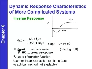
slope. If ….fast response. : zero of transfer function. Dynamic Response Characteristics of More Complicated Systems. Inverse Response. Chapter 6. (see Fig. 6.3). Use nonlinear regression for fitting data (graphical method not available). Chapter 6. Chapter 6.

Inverse Response
E N D
Presentation Transcript
slope If ….fast response : zero of transfer function Dynamic Response Characteristics of More Complicated Systems Inverse Response Chapter 6 (see Fig. 6.3) Use nonlinear regression for fitting data (graphical method not available)
Chapter 6 For inverse response
Chapter 6 4 poles (denominator is 4th order polynomial)
More General Transfer Function Models • Poles and Zeros: • The dynamic behavior of a transfer function model can be characterized by the numerical value of its poles and zeros. • General Representation of a TF: • There are two equivalent representations: Chapter 6
where {zi} are the “zeros” and {pi} are the “poles”. • We will assume that there are no “pole-zero” cancellations. That is, that no pole has the same numerical value as a zero. • Review: in order to have a physically realizable system. Chapter 6
Time Delays Time delays occur due to: • Fluid flow in a pipe • Transport of solid material (e.g., conveyor belt) • Chemical analysis • Sampling line delay • Time required to do the analysis (e.g., on-line gas chromatograph) Chapter 6 Mathematical description: A time delay, , between an input u and an output y results in the following expression:
Chapter 6 H1/Qi has numerator dynamics (see 6-72)
Approximation of Higher-Order Transfer Functions In this section, we present a general approach for approximating high-order transfer function models with lower-order models that have similar dynamic and steady-state characteristics. In Eq. 6-4 we showed that the transfer function for a time delay can be expressed as a Taylor series expansion. For small values of s, Chapter 6
An alternative first-order approximation consists of the transfer function, Chapter 6 • where the time constant has a value of • These expressions can be used to approximate the pole or zero term in a transfer function.
Skogestad’s “half rule” • Skogestad (2002) has proposed an approximation method for higher-order models that contain multiple time constants. • He approximates the largest neglected time constant in the following manner. • - One half of its value is added to the existing time delay (if any) and the other half is added to the smallest retained time constant. • - Time constants that are smaller than the “largest neglected time constant” are approximated as time delays using (6-58). Chapter 6
Example 6.4 Consider a transfer function: Derive an approximate first-order-plus-time-delay model, Chapter 6 • using two methods: • The Taylor series expansions of Eqs. 6-57 and 6-58. • Skogestad’s half rule Compare the normalized responses of G(s) and the approximate models for a unit step input.
Solution • The dominant time constant (5) is retained. Applying • the approximations in (6-57) and (6-58) gives: and Chapter 6 Substitution into (6-59) gives the Taylor series approximation,
(b) To use Skogestad’s method, we note that the largest neglected time constant in (6-59) has a value of three. • According to his “half rule”, half of this value is added to the next largest time constant to generate a new time constant • The other half provides a new time delay of 0.5(3) = 1.5. • The approximation of the RHP zero in (6-61) provides an additional time delay of 0.1. • Approximating the smallest time constant of 0.5 in (6-59) by (6-58) produces an additional time delay of 0.5. • Thus the total time delay in (6-60) is, Chapter 6
and G(s) can be approximated as: The normalized step responses for G(s) and the two approximate models are shown in Fig. 6.10. Skogestad’s method provides better agreement with the actual response. Chapter 6 Figure 6.10 Comparison of the actual and approximate models for Example 6.4.
Multivariable Processes many examples: distillation columns, FCC, boilers, etc. Consider stirred tank with level controller Chapter 6 2 disturbances (Ti, wi) 2 control valves (A, B) manipulate ws, wo 2 measurements (T0, h) controlled variables (T0, h) change in w0 affects T0 and h change in ws only affects T0
Three non-zero transfer functions Transfer Function Matrix Chapter 6 From material and energy balances,
Chapter 6 Normal method, but interactions may present tuning problems. In multivariable control, interactions are treated, but controller design is more complicated.
Chapter 6 Previous chapter Next chapter