Learn Logarithmic Functions & Properties
Understand how logarithmic functions work, including the natural logarithm, inverse relationships, and properties. Solve examples and explore the properties of logarithms.


Learn Logarithmic Functions & Properties
E N D
Presentation Transcript
7 INVERSE FUNCTIONS
INVERSE FUNCTIONS 7.3 Logarithmic Functions • In this section, we will learn about: • Logarithmic functions and natural logarithms.
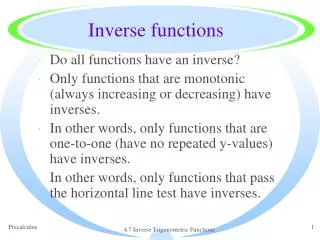
LOGARITHMIC FUNCTIONS • If a > 0 and a≠ 1, the exponential function • f(x) = ax is either increasing or decreasing, • so it is one-to-one. • Thus, it has an inverse function f-1, which • is called the logarithmic function with base a • and is denoted by loga.
LOGARITHMIC FUNCTIONS Definition 1 • If we use the formulation of an inverse • function given by (7.1.3), • then we have:
LOGARITHMIC FUNCTIONS • Thus, if x > 0, then logax is the exponent • to which the base a must be raised • to give x.
LOGARITHMIC FUNCTIONS Example 1 • Evaluate: • log381 • log255 • log100.001
LOGARITHMIC FUNCTIONS Example 1 • log381 = 4 since 34 = 81 • log255 = ½ since 251/2 = 5 • log100.001 = -3 since 10-3 = 0.001
LOGARITHMIC FUNCTIONS Definition 2 • The cancellation equations (Equations 4 in Section 7.1), when applied to the functions f(x) = axand f -1(x) = logax, become:
LOGARITHMIC FUNCTIONS • The logarithmic function logahas domain and range . • It is continuous since it is the inverse of a continuous function, namely, the exponential function. • Its graph is the reflection of the graph of y = ax about the line y = x.
LOGARITHMIC FUNCTIONS • The figure shows the case where • a > 1. • The most important logarithmic functions have base a > 1.
LOGARITHMIC FUNCTIONS • The fact that y = ax is a very rapidly • increasing function for x > 0 is reflected in the • fact that y = logax is a very slowly increasing • function for x > 1.
LOGARITHMIC FUNCTIONS • The figure shows the graphs of y = logax • with various values of the base a > 1. • Since loga1 = 0, the graphs of all logarithmic functions pass through the point (1, 0).
LOGARITHMIC FUNCTIONS • The following theorem summarizes the properties of logarithmic functions.
PROPERTIES OF LOGARITHMS Theorem 3 • If a > 1, the function f(x) = logax isa one-to-one, continuous, increasing function with domain (0, ∞) and range . • If x, y > 0 and r is any real number, then
PROPERTIES OF LOGARITHMS • Properties 1, 2, and 3 follow from the corresponding properties of exponential functions given in Section 7.2
PROPERTIES OF LOGARITHMS Example 2 • Use the properties of logarithms in Theorem 3 to evaluate: • log42 + log432 • (b) log280 - log25
PROPERTIES OF LOGARITHMS Example 2 a • Using Property 1 in Theorem 3, we have: • This is because 43 = 64.
PROPERTIES OF LOGARITHMS Example 2 b • Using Property 2, we have: • This is because 24 = 16.
LIMITS OFLOGARITHMS • The limits of exponential functions given in Section 7.2 are reflected in the following • limits of logarithmic functions. • Compare these with this earlier figure.
LIMITS OFLOGARITHMS Equation 4 • If a > 1, then • In particular, the y-axis is a vertical asymptote of the curve y = logax.
LIMITS OFLOGARITHMS Example 3 • As x → 0, we know that t = tan2x→ tan20 = 0and the values of t are positive. • Hence, by Equation 4 with a = 10 > 1, we have:
NATURAL LOGARITHMS • Of all possible bases a for logarithms, • we will see in Chapter 3 that the most • convenient choice of a base is the number e, • which was defined in Section 7.2.
NATURAL LOGARITHMS • The logarithm with base e is called • the natural logarithm and has a special • notation:
NATURAL LOGARITHMS Definitions 5 and 6 • If we put a = e and replace loge with ‘ln’ • in (1) and (2), then the defining properties of • the natural logarithm function become:
NATURAL LOGARITHMS • In particular, if we set x = 1, • we get:
NATURAL LOGARITHMS E. g. 4—Solution 1 • Find x if ln x = 5. • From (5), we see thatln x = 5 means e5 = x • Therefore, x = e5.
NATURAL LOGARITHMS E. g. 4—Solution 1 • If you have trouble working with the ‘ln’ • notation, just replace it by loge. • Then, the equation becomes loge x = 5. • So, by the definition of logarithm, e5 = x.
NATURAL LOGARITHMS E. g. 4—Solution 2 • Start with the equation ln x = 5. • Then, apply the exponential function to both • sides of the equation: eln x= e5 • However, the second cancellation equation in Equation 6 states that eln x = x. • Therefore, x = e5.
NATURAL LOGARITHMS Example 5 • Solve the equation e5 - 3x = 10. • We take natural logarithms of both sides of the equation and use Definition 9: • As the natural logarithm is found on scientific calculators, we can approximate the solution—to four decimal places: x≈ 0.8991
NATURAL LOGARITHMS Example 6 • Express as a single • logarithm. • Using Properties 3 and 1 of logarithms, we have:
NATURAL LOGARITHMS • The following formula shows that • logarithms with any base can be • expressed in terms of the natural • logarithm.
CHANGE OF BASE FORMULA Formula 7 • For any positive number a (a≠ 1), • we have:
CHANGE OF BASE FORMULA Proof • Let y = logax. • Then, from (1), we have ay= x. • Taking natural logarithms of both sides of this equation, we get yln a = ln x. • Therefore,
NATURAL LOGARITHMS • Scientific calculators have a key for • natural logarithms. • So, Formula 7 enables us to use a calculator to compute a logarithm with any base—as shown in the following example. • Similarly, Formula 7 allows us to graph any logarithmic function on a graphing calculator or computer.
NATURAL LOGARITHMS Example 7 • Evaluate log8 5 correct to six • decimal places. • Formula 7 gives:
NATURAL LOGARITHMS • The graphs of the exponential function y = ex • and its inverse function, the natural logarithm • function, are shown. • As the curve y = excrosses the y-axis with a slope of 1, it follows that the reflected curve y = ln x crosses the x-axis with a slope of 1.
NATURAL LOGARITHMS • In common with all other logarithmic functions • with base greater than 1, the natural • logarithm is a continuous, increasing function • defined on and the y-axis is • a vertical asymptote.
NATURAL LOGARITHMS Equation 8 • If we put a = e in Equation 4, then we have these limits:
NATURAL LOGARITHMS Example 8 • Sketch the graph of the function • y = ln(x - 2) -1. • We start with the graph of y = ln x.
NATURAL LOGARITHMS Example 8 • Using the transformations of Section 1.3, we shift it 2 units to the right—to get the graph of y = ln(x - 2).
NATURAL LOGARITHMS Example 8 • Then, we shift it 1 unit downward—to get the graph of y = ln(x - 2) -1. • Notice that the line x = 2 is a vertical asymptote since:
NATURAL LOGARITHMS • We have seen that ln x → ∞ as x → ∞. • However, this happens veryslowly. • In fact, ln x grows more slowly than any positive power of x.
NATURAL LOGARITHMS • To illustrate this fact, we compare • approximate values of the functions • y = ln x and y = x½= in the table.
NATURAL LOGARITHMS • We graph the functions here. • Initially, the graphs grow at comparable rates. • Eventually, though, the root function far surpasses the logarithm.
NATURAL LOGARITHMS • In fact, we will be able to show in Section 7.8 that: for any positive power p. • So, for large x, the values of ln x are very small compared with xp.