Chapter 6 Section 3

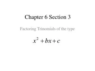
Chapter 6 Section 3 Assignment of Probabilities

Sample Space and Probabilities • Sample Space : S = { s1 , s2 , s3 , … , sN-1 , sN } where s1 , s2 , s3 , … , sN-1 , sN are all the possible outcomes of the experiment • Each outcome can be assigned a number that represents the probability of an outcome.

Probability Distribution

Fundamental Properties of Probability Distributions • 0 < p1 < 1 0 < p2 < 1 0 < p3 < 1 0 < pN < 1 2. p1 + p2 + p3 + … + pN-1 + pN = 1

Assigning Probabilities • Theoretically • Using Logic and/or Counting Techniques • Best method for assigning probabilities • See Example 1 & 2 on page 273 • Empirically (i.e. Experimentally) • Works only when the observed trial are representative of the sample space. • See Example 3 on pages 273 and 274

Exercise 3 (page 281) • Red die and green die are tossed and the number of the side facing up are observed. • Sample Space: S = { (1,1), (1,2), (1,3), (1,4), (1,5), (1,6), (2,1), (2,2), (2,3), (2,4), (2,5), (2,6), (3,1), (3,2), (3,3), (3,4), (3,5), (3,6), (4,1), (4,2), (4,3), (4,4), (4,5), (4,6), (5,1), (5,2), (5,3), (5,4), (5,5), (5,6), (6,1), (6,2), (6,3), (6,4), (6,5), (6,6) }

Exercise 3 continued • Note that each pair is equally likely to be picked if we randomly select a pair, thus the probability distribution is: OutcomeProbability s1 = (1,1) p1 = 1/36 s2 = (1,2) p2 = 1/36 s3 = (1,3) p3 = 1/36 s36 = (6,6) p36 = 1/36

Addition Principle • Let the event E be defined as E = { s , t , u , … , z } Then Pr( E ) = Pr(s) + Pr(t) + Pr(u) + … + Pr(z)

Exercise 3 Part (a) • Let E = {‘the numbers add up to 8’} • E = { (2,6) , (3,5) , (4,4) , (5,3) , (6,2) } • Find the Pr( E ) • Pr( E ) = Pr( (2,6) ) + Pr( (3,5) ) + Pr( (4,4) ) + Pr( (5,3) ) + Pr( (6,2) ) • Pr( E ) = 1/36 + 1/36 + 1/36 + 1/36 + 1/36 = 5/36  0.1389

Inclusion – Exclusion Principle as Applied to Probabilities • Let E and F be events, then Pr( E  F ) = Pr ( E ) + Pr ( F ) – Pr( E  F ) Venn Diagrams and Probabilities We can use Venn Diagrams and place numbers that represent the probability that the elements in the basic region will occur.

Exercise 17 (page 282) • Let E and F be events. • Pr( E ) = 0.6 , Pr( F ) = 0.5 , and Pr( E  F ) = 0.4 (a) Find Pr( E  F ) (b) Find Pr( E  F)

Odds • When the odds in favor of an event a to b , then the probability of the event can be found by p = a / ( a + b ) • a represents the number of times that the event occurs • b represents the number of times that the event does not occur

Converting an Odds to a Probability • Example: If the odds of a horse to win a race is 1 to 60, then then probability of the horse winning is: a = 1 and b = 60 p = a / (a + b) = 1 / (1 + 60) = 1/61  0.0164

Converting a Probability to an Odds • List the probability as a decimal number • Convert the decimal number to a fraction. • Reduce the fraction (when possible). • Split the value in the denominator to the sum of two values, where the first value in the sum is the value in the numerator. • Get the values of a and b from the resulting fraction.

Chapter 6 Section 3