Download

1 / 23
250 likes | 395 Views
Mean Delay in M/G/1 Queues with Head-of-Line Priority Service and Embedded Markov Chains. Wade Trappe. Lecture Overview. Priority Service Setup Mean Waiting Time for Type-1 Mean Waiting Time for Type-2 Generalization Summary Embedded Markov Chain Technique N k inside of N(t)

E N D
Mean Delay in M/G/1 Queues with Head-of-Line Priority ServiceandEmbedded Markov Chains Wade Trappe
Lecture Overview • Priority Service • Setup • Mean Waiting Time for Type-1 • Mean Waiting Time for Type-2 • Generalization • Summary • Embedded Markov Chain Technique • Nk inside of N(t) • The queue distribution for M/G/1 • The PGF approach • Example: M/H2/1 Queue • Homework: Alternate Pollaczek-Khinchine Derivation
M/G/1 Priority Services: Setup • Consider a queue that handles K priority classes of customers • Type-k customers arrive as a Poisson Process with rate and service times according to . • Customers are separated as they arrive and assigned to different “prioritized” queues • Each time the server is free: • Selects the next customer from highest priority, non-empty queue • This is the “head of line” service • We also assume that customers are not pre-empted! • Server Utilization for type-k customers is • Stability requirement:
Priority Services: Explanation 1 1 Queue-1 1 Server 2 2 Queue-2 Blue Type-1 Packets always have priority, but cannot preempt Type-2 packets
Priority Services: Mean Waiting Times • Our first goal will be to calculate the mean waiting time for Type-1 customers, i.e. • Assume a type-1 customer arrives and finds Nq1(t)=k1 type-1 already in the queue • Assume we use FCFS within each class • W1 consists of: • Residual time R of customer in server • k1 service times of type-1 in queue • Thus: • We get the mean waiting time for type-1 as
Priority Services: Mean Waiting Times, pg 2 • Now, let us look at a type-2 customer. When he arrives he may find • Nq1(t)=k1 type-1 already in the queue-1 • Nq2(t)=k2 type-2 already in the queue-2 • Thus, W2 is the sum of: • Residual service time R • k1 service times for type-1customers • k2 service times for type-2 customers • AND service times of any new type-1 customers!!! • We get the mean waiting time for type-2 as
Priority Services: Mean Waiting Times, pg 3 • Here, M1 is the number of customers of type-1 that arrive during type-2’s waiting period • By Little’s Theorem applied to the queues: • The mean number of type-1 arrivals during seconds is • Substitute to get
Priority Services: Mean Waiting Times, pg 4 • Solve for : • Generalizing gives • Now, we’re left with finding E[R]!
Priority Services: Mean Waiting Times, pg 5 • When a customer arrives, the one being serviced can be of any type! So R must account for this! • We will use the same formulation as where is the aggregate Poisson Process rate. • To get E[X2] we use the fact that the fraction of type-k customers is : • Thus, we get
Priority Services: Mean Delay • Now, calculating the mean delay for a type-k customer is easy! • From this, observe: • Class-k customers are affected by the behavior of lower priority customers
The Embedded Markov Chain Nk Nk-2 Nk-1 • Let Nk be the number of customers found in the system just after the service completion of the k-th customer • Let Ak be the number of customers who arrive while the k-th customer is served • The Ak are i.i.d. • Under FCFS: Ak is independent of N1, N2, …, Nk-1 • Nk is not independent of Ak N(t) Time Ck-2 Ck-1 Ck Xk-1 Xk Service Ck-1 Ck Queue Ck-1 Ck Ck+1 Ak-1=1 Ak=3
Embedded Markov Chain, pg 2 • We may find the following recursion: • Where did first line come from? • If , then k-th customer finds the system empty, and on departure he leaves behind those who have arrived during his service. • The second line: • The queue left by the k-th customer consists of the previous queue decreased by one plus the new arrivals during his service. • Let U(x)=1 for x>0 and U(x)=0 for x<=0 • Then we get
Embedded Markov Chain, pg 3 • From we can see that Nk is a Markov Chain since Nk depends on the past only through Nk-1 • Nk is called the embedded Markov Chain • (Homework): The distribution for N(t) and Nk are the same: • Step 1: Show, in M/G/1, distributions found by arriving customers is the same as that left by departing customers • Step 2: Show, in M/G/1, the distribution of customers found by arriving customers is the same as the steady state distribution of N(t) • We will analyze Nk instead of N(t)
M/G/1 Queue Distribution • To find the queue distribution, we use the probability generating function method • The PGF of the distribution {pn} is • Substitute and use independence to get • Thus
M/G/1 Queue Distribution, pg. 2 • If the service time of customer k is t, then Ak has a Poisson distribution with mean lt • Now multiply by the fX(t), the pdf of the service time Xk, This gives the joint distribution. • Integrate out X to obtain the unconditional pdf of Ak • What does this remind you of? • Answer: Laplace Transforms!!!
M/G/1 Queue Distribution, pg. 3 • The Probability Generating Function of Ak is given by • Substitute into earlier result to get: Laplace Transform of fX(t)
Show This! M/G/1 Queue Distribution, pg. 4 • We need to now find p0! • To do this, look at limit as z goes to 1, and apply L’Hopital… • First, go back to • Observe that P(z=1)=1, Ak(z=1)=1 • Thus • We used:
M/G/1 Queue Distribution, pg. 5 • Thus, • This is exactly what we got for M/M/1 Queues!!! • Substitute into earlier result to get: • What do we do with this? Use it to find the probability distribution pn! • How? Equate terms… Best to see an example
M/H2/1 Queue • Consider the case where FX(t), the cdf, is a two-term hyper-exponential distribution: • Where do hyper-exponentials come from? • In practice, from situations where service times can be represented as a mixture of exponential distributions… • That is, suppose there are k types of customers, each occuring with a probability pi (so sum = 1) • Customer of type I has a service time exponentially distributed with mean 1/mi • Then the density is
M/H2/1 Queue, pg. 2 • Back to our 2-phase hyper-exponential problem… • The mean service time is given by • The Laplace Transform of fX(t) is: • We thus get:
M/H2/1 Queue, pg. 3 • The PGF of {pn} is • The probability distribution is obtained through partial-fraction expansion of P(z). • To do this, we must find the roots of the denominator… call these z1 and z2 • Then P(z) has the form: = Total Traffic Intensity
M/H2/1 Queue, pg. 4 • Solving for C1 and C2 involves setting z=0 and z=1 to get • Finally, upon substitution, we get: