Download

1 / 18
180 likes | 203 Views
Learn the difference between queues and priority queues (Heaps), complexity of Heaps, and applications in OS and sorting algorithms. Explore simple and advanced implementations like linked lists, binary search trees, and binary heaps. Understand the structure and order properties of Heaps for optimal performance.

E N D
Chapter (6) Priority Queues (Heaps) The goals: Efficient implementation of the ADT priority queue. Application of priority queues. Advanced implementations of priority queues. Questions: What is the difference between queues and priority queues (Heaps)? What is the complexity of Heaps? Heap is, in some ways, like binary search tree. The entry contained by a node is greater than or equal to the entries of the node’s children. The tree is a complete binary tree, so every level except the deepest must contain as many nodes as possible. In addition, in the deepest level, all the nodes are as far left as possible.
Jobs sent to a line printer are generally placed on a queue. But this may not be the best thing to do. For instance, one job may be particularly more important than others. Thus, we need to let that job gets processed as soon as the printer becomes available. In a multi-user environment, the operating system scheduler must decide which of the several processes to run. Generally a process is allowed to run for a fixed period of time. All jobs go on the queue, and scheduler takes the first job from the queue and run it until either the job is finished or until the time limit is up. If the job is not finished that job will be placed at the end of queue. This is not an appropriate strategy. In this case short jobs will take a long time to run because of wait involved to run. In general, it is important that the short jobs finish as fast as possible. Thus, these jobs have preference over jobs that are already been running. Furthermore, some jobs that are not short but are very important will have preference too.
Model Priority queue is an ADT that allows at least: the Insert and Delete_Min. We know what insert’s job is, Delete_Min finds, passes back, and removes the minimum element in the priority queue. The Insert operator is equivalent of Enqueue, and Delete_Min is the priority queue equivalent of the queue’s of the Dequeue operation. We may add other operators to this ADT. Priority queue have applications in: operating systems, external sorting, and are important in the implementation of the greedy algorithm.
Simple Implementations 1) Linked list: performing insertions at the front is O(1) and traversing the list to delete the minimum in O(n) time. If we keep the list sorted, insertion becomes expensive O(n) and Delete_Mins cheap. Since there are never more Delete_Mins than insertions, it is better to make the insertion cheaper. Thus, it is better to use the first method. 2) Binary search tree: This gives an O(logn) average running time for both operations. Although, the insertions are random and the deletion are not, this is always true. Problem with this method is that repeatedly removing a node form left subtree makes the tree imbalance. In general, in the worse case, the right subtree may end up having twice as elements as it should. This adds only a small constant to the expected depth. We can make the bound into a worst-case bound by using a balanced tree. This protect one against bad insertion sequence. Using binary search tree could be overkill. BST supports more operations that is needed for Heaps.
Binary Heap This is the most common way of implementing Heaps. Like a binary search tree, heaps have two properties: 1) a structure property, and 2) a heap order property. As with AVL trees, an operation on a heap can destroy one of the properties, so a heap operation must not terminate until all heap properties are in order. Structure Property A heap is a binary tree that is completely filled, with the possible exception of the bottom level, which is filled from left to right. Such a tree is known as a Complete Binary Tree.
We can show that a complete binary tree of height h has between 2hand 2h+1-1 nodes. This implies that the height of a complete binary tree is: This is clearly O(logn). Important note: A complete binary tree is so regular, that it can be represented in an array and no pointers are necessary. The following array corresponds to the tree that is shown below. For any element in the array position i, the left child is in position 2i, the right child is in the cell after the left child (2i + 1), and the parent is in position . Thus, we not only do not need pointers, but the operations required to traverse the tree are extremely simple and fast. The only problem is estimating the maximum heap size required, in advance. This is not a major problem. So a heap structure consists of an array (of desired type) and an integer representing the current heap size.
Heap Order Property The property that allows operations to be performed quickly is the heap order property. Our concern is to find the minimum quickly. Thus, it make sense that the smallest element should be at the root. If we consider that, then any subtree also should be a heap. That means any node should be smaller than all of its descendants. Heap Order Property: In a heap, for every node X, the key in the parent of X is smaller than (or equal to) the key in X, with the obvious exception of the root. By this order, the minimum element can always be found at the root, this means that we get the extra operation, Find_Min, in constant time.
Basic heap Operations • Insert: • Here is the steps: • Insert X at the bottom level at the next available location. Otherwise the tree will not be complete. • If the heap order is not violated, keep X there. Otherwise, • Slide the element up toward the root and slide the upper node down in place of X. Continue this process until you are in the correct location. • This general strategy is called percolate up: which means the new element is percolated up the heap until the correct location is found.
If the new element to be inserted is a new minimum, it will be pushed all the way to the top. The time to do the insertion could be as much as O(logn) if the element to be inserted is the new minimum and is percolated all the way to the root. It is shown that on average, 2.607 comparisons are required to perform an insert, so the average Insert moves an element up 1.067 levels.
Delete_Min Procedure for this operation is very similar to that of Insertion. Finding the minimum is easy, removing it is the hard part. Here are the steps for removal: 1) remove the root, that is the minimum, 2) Move the value in the last location (last inserted) to the root location. 3) If that value is valid at that location, do nothing, otherwise 4) percolate down until you find the correct location for the moved key.
The worst-case running time for this operation is O(logn). On average, the element that is placed at the root is percolated almost to the bottom of the heap, where it has come from, so the average running time is O(logn).
A heap is excellent for finding minimum, in fact finding minimum will be an O(1) operation. However, using a heap to find max is of no help. Heap has a very little ordering. So there is no way to find a particular key without a linear scanning of the entire heap. If you want to know where everything is, then you have to use some other data structure, such as a hash table, in addition to heap. If we assume that we know the position of every element, then the following operations will run in logarithmic worst-case time. Decrease_Key: The operations lowers the value of the key at position P by a positive amount . This may violate the heap order, thus, it must be fixed by a percolate up. This is a very powerful technique for administrators, they can lower their key to their jobs run with highest priority. Increase_Key: The operation increases the value of the key at position P by a positive amount . This is done using percolate down. Many schedulers automatically drop the priority of a process that is consuming excessive CPU time. Remove: The Remove(I) operation removes the node at position I from the heap. This is done by first performing and then performing Delete_Min. When a process is terminated by a user (instead of normally finishing), it must be removed from the priority queue. Build_Heap: The Build_Heap operation takes as input n keys and places them into an empty heap. Obviously, this can be done with n successive Insert. Since, every Insert will take O(1) average and O(logn) worst-case time, the total running time of this algorithm would be O(n) average but O(nlogn) worst-case.
General algorithm is to place the n keys into the tree in any order, maintaining the structure property. Then, if Percolate_Down(P) percolates down from node P, perform the algorithm below (Figure 6.14) to create a heap-ordered tree. for( i = N/2; i > 0, i--) Percolate_Down( i ); Example: The tree shown here is not a heap-ordered. We used the above algorithm to order it. In this tree, N = 15, we could compute that using the height of the tree. Note that the height is 3 and the tree is full, based on the theory That we proved previously, this tree should have 2h+1-1 nodes, or 23+1 - 1 = 15 nodes. You will observe that the root is not the minimum, and some of the keys at the bottom part of the tree have lower values than the keys at the top portion. What is the array corresponding to this tree? 150 80 40 30 10 70 110 100 20 90 60 50 120 140 130 Index: 0 1 2 3 4 5 6 7 8 9 10 11 12 13 14 15
Based on the algorithm given in the previous page, the for loop starts from N/2 = 15/2 =7 and goes down to 0. Thus, these are the values that we will see for i: 7, 6, 5, 4, 3, 2, 1. i = N/2 = 7 i =5 i = 6
i =3 i =4 i =1 i =2
There were 10 dashed lines in the tree corresponding to 20 comparisons. In order to bound the running time of Build_Heap, we must bound the number of dashed lines. This can be done by computing the sum of the heights of all the nodes in the heap. This is the maximum of dashed lines. The best thing is to show that this sum is O(n). For the perfect binary tree of height h containing 2h+1-1 nodes, the sum of the height of the nodes is 2h+1-1-(h+1). Important: prove it on your own ...
Applications: The selection Problem: Remember in chapter (1) we had a problem where we wanted to select the kth largest element. Two algorithms were given in that chapter. A) To sort the list and return the kth value. Assuming a simple sort that was an O(n2) complexity. B) To read k elements into an array and sort them, then read the rest of the elements one-by-one. If an element larger than the last member was found place it in the appropriate location and drop the kth element from the array. At the end return the kth element. Best case for this algorithm is O(n.k) and worst case is O(n2). Using heap we can do this more efficiently. Algorithm 6A: Use Build_heap to build the tree, then perform kDelete_Min operations. The last element extracted from the heap is our answer. The worst-case timing is O(n) to reconstruct the heap using Build_Heap and O(logn) for each Delete_Min. Since we have k Delete_Mins, the total running time is: O(n + klogn). Now, if k=O(n/logn), then the running time is dominated by the Build_Heap operation and it will be: O(n). For the larger values of k, the running time is O(klogn). If , then we will have:
Algorithm 6B: This is the same as the second algorithm in Chapter (1). Here we keep k elements and will follow the same procedure, but we use heap to implement the algorithm. We will maintain a set S of the k largest elements. Of course, if that is an ordered heap, we will see the minimum at the root. Now, we look at the rest of numbers one-by-one. If there is something larger than the root, we place it at the root and we re_order to make sure the smallest key stays at root. We continue this process until all keys are read. At the end the root will be the kth element. Here is some words on the complexity: The first k elements are placed into the heap in total time O(k) with a call to Build_heap. The time to process each of the remaining elements is O(1) and to test if the element goes to the heap (compare with the root only), Then we have an O(logk) to delete Sk and insert the new element. Total is: O(k + (n-k) logk) = O(nlogk). This algorithm will give a bound of: for finding median.