Download
1 / 47
470 likes | 511 Views
Understand the fundamentals of quantum theory systems and subsystems, distinguishing between closed and open systems, concrete versus abstract systems, and different types of system descriptions in classical and quantum physics. Learn about states and state spaces, distinguishability of states, state vectors, and Hilbert space in quantum mechanics.

E N D
Systems and Subsystems • Intuitively speaking, a physical system consists of a region of spacetime & all the entities (e.g. particles & fields) contained within it. • The universe (over all time) is a physical system • Transistors, computers, people: also phys. systs. • One physical system A is a subsystem of another system B (write AB) iff A is completely contained within B. • Later, we may try to make these definitions more formal & precise. B A
Closed vs. Open Systems • A subsystem is closed to the extent that no particles, information, energy, or entropy (terms to be defined) enter or leave the system. • The universe is (presumably) a closed system. • Subsystems of the universe may be almost closed • Often in physics we consider statements about closed systems. • These statements may often be perfectly true only in a perfectly closed system. • However, they will often also be approximately true in any nearly closed system (in a well-defined way)
Concrete vs. Abstract Systems • Usually, when reasoning about or interacting with a system, an entity (e.g. a physicist) has in mind a description of the system. • A description that contains every property of the system is an exact or concrete description. • That system (to the entity) is a concrete system. • Other descriptions are abstract descriptions. • The system (as considered by that entity) is an abstract system, to some degree. • We nearly always deal with abstract systems! • Based on the descriptions that are available to us.
System Descriptions • Classical physics: • A system could be completely described by giving a single state S out of the set of all possible states. • Statistical mechanics: • Instead, give a probability distribution functionp:[0,1] stating that the system is in state S with probability p(S). • Quantum mechanics: • Give a complex-valued wavefunction: ℂ, |(S)|1, implying the system is instate S with probability |(S)|2.
States & State Spaces • A possible stateS of an abstract system A (described by a description D) is any concrete system C that is consistent with D. • I.e., it is possible that the system in question could be completely described by the description of C. • The state space of A is the set of all possible states of A. • So far, the concepts we’ve discussed can be applied to either classical or quantum physics • Now, let’s get to the uniquely quantum stuff…
Distinguishability of States • Classical & quantum mechanics differ crucially regarding the distinguishability of states. • In classical mechanics, there is no issue: • Any two states s,t are either the same (s=t), or different (st), and that’s all there is to it. • In quantum mechanics (i.e. in reality): • There are pairs of states st that are mathematically distinct, but not 100% physically distinguishable. • Such states cannot be reliably distinguished by any number of measurements, no matter how precise. • But you can know the real state (with high probability), if you prepared the system to be in a certain state.
State Vectors & Hilbert Space • Let S be any maximal set of distinguishable possible states s, t, … of an abstract system A. • I.e., no possible state that is not in S is perfectly distinguishable from all members of S. • Identify the elements of S with unit-length, mutually-orthogonal (basis) vectors in an abstract complex vector space ℋ. • The system’s “Hilbert space” • Postulate 1: Each possible state ofsystem A can be identified with a unit-length vector in the Hilbert space ℋ. t s
(Abstract) Vector Spaces • A concept from abstract linear algebra. • A vector space, in the abstract, is any set of objects that can be combined like vectors, i.e.: • You can add them • Addition is associative & commutative • Identity law holds for addition to zero vector 0 • You can multiply them by scalars (incl. 1) • Associative, commutative, and distributive laws hold • Note: There is no inherent basis (set of axes) • The vectors themselves are the fundamental objects,rather than being just lists of coordinates
Hilbert spaces • A Hilbert spaceℋ is a vector space in which the scalars are complex numbers, with an inner product (dot product) operation : ℋ×ℋ C • See Hirvensalo p. 107 for defn. of inner product: xy = (yx)* (* = complex conjugate) xx 0 xx= 0 if and only if x = 0 xy is linear, under scalar multiplication and vector addition within both x and y “Component”picture: y Another notation often used: x xy/|x| “bracket”
Review: The Complex Number System • It is the extension of the real number system via closure under exponentiation. • (Complex) conjugate: c* = (a + bi)* (a bi) • Magnitude or absolute value: |c|2= c*c =a2+b2 +i The “imaginary”unit c b + a “Real” axis “Imaginary”axis i
Review: Complex Exponentiation • Powers of i are complex units: • Note: ei/2 = i ei= 1 e3 i/2 = i e2 i= e0 = 1 ei +i 1 +1 i
Vector Representation of States • Let S={s0, s1, …} be any maximal set of mutually distinguishable states, indexed by i. • A basis vector vi identified with the ith such state can be represented as a list of numbers: s0s1s2si-1si si+1 vi = (0, 0, 0, …, 0, 1, 0, … ) • Arbitrary vectors v in the Hilbert space ℋ can then be defined by linear combinations of the vi: • And the inner product is given by:
Dirac’s Ket Notation • Note: The inner product definition is the same as the matrix product of x, as a conjugated row vector, times y, as a normal column vector. • This leads to the definition, for state s, of: • The “bra” s| means the row matrix [c0* c1* …] • The “ket” |s means the column matrix • The adjoint operator † takes any matrix Mto its conjugate transpose M†MT*, sos| can be defined as |s†, and xy = x†y. “Bracket”
Distinguishability of States, again • State vectors s and t are (perfectly) distinguishable or orthogonal (write st) iff s†t = 0. (Their inner product is zero.) • State vectors s and t are perfectly indistinguishable or identical (write s=t) iff s†t = 1. (Their inner product is one.) • Otherwise, s and t are both non-orthogonal, andnon-identical. Not perfectly distinguishable. • We say, “the amplitude of state s, given state t, is s†t”. Note: amplitudes are complex numbers.
Probability and Measurement • A yes/no measurement is an interaction designed to determine whether a given system is in a certain state s. • The amplitude of state s, given the actual state t of the system determines the probability of getting a “yes” from the measurement. • Postulate 2: For a system prepared in state t,any measurement that asks “is it in state s?” will say “yes” with probability P(s|t) = |s†t|2 • After the measurement, the state is changed, in a way we will define later.
A Simple Example • Suppose abstract system S has a set of only 4 distinguishable possible states, which we’ll call s0, s1, s2, and s3, with corresponding ket vectors |s0, |s1, |s2, and |s0. • Another possible state is then the unit vector • Which is equal to the column matrix: • If measured to see if it is in state s0, we have a 50% chance of getting a “yes”.
Linear Operators • V,W: Vector spaces. • A linear operator A from V to W is a linear function A:VW. An operator onV is an operator from V to itself. • Given bases for V and W, we can represent linear operators as matrices. • An Hermitian operator H on V is a linear operator that is self-adjoint (H=H†). • Its diagonal elements are real.
Eigenvalues & Eigenvectors • v is called an eigenvector of linear operator A iff A just multiplies v by a scalar a, i.e.Av=av • “eigen” (German) means “characteristic” • a, the eigenvalue corresponding to eigenvectorv, is just the scalar that A multiplies v by • a is degenerate if it is shared by 2 eigenvectors that are not scalar multiples of each other • Any Hermitian operator has all real-valued eigenvectors, which form an orthogonal set
Observables • A Hermitian operator H on the set V is called an observable if there is an orthonormal (all unit-length, and mutually orthogonal) subset of its eigenvectors that forms a basis of V. • Postulate 3: Every measurable physical property of a system can be described by a corresponding observable H. Measurement outcomes correspond to eigenvalues of H. • The measurement can also be thought of as a yes-no test that compares the state with each of the observable’s normalized eigenvectors.
Wavefunctions • Given any set Sℋ of system states, • Whether all mutually distinguishable, or not, • a quantum state vector v can be translated to a wavefunction:Sℂ, giving, for each state sS, the amplitude (s) of that state. • When s is some other state vector, and the “actual” state is v, then (s) is just s†v. • Whenever S includes a basis set, determines v. • is called a “wavefunction” because its dynamics takes the form of a wave equation when S ranges over a space of positional states.
Time Evolution • Postulate 4: (Closed) systems evolve (change state) over time via unitary transformations. t2 = Ut1t2t1 • Note that since U is linear, a small-factor change in the amplitude of a particular state at t1 leads to a correspondingly small change in the amplitude of the corresponding state at t2! • Chaotic sensitivity to initial conditions requires an ensemble of initial states that are different enough to be distinguishable (in the sense we defined) • Indistinguishable initial states never beget distinguishable outcomes true chaotic/analog computing doesn’t exist
Schrödinger's Wave Equation • Start w. classical Hamiltonian energy equation:H = K + P (K = kinetic, P = potential) • Express K in terms of momentum:K = ½mv2 = p2/2m • Substitute H = i∂/t and p = i∂/x: • Apply to wavefunction Ψ over position states x: (Where ∂/a≝ ∂/∂a)
Multidimensional Form For a system with states given by(x,t) where t is a global time coordinate, and xdescribes N/3 particles (p0,…,pN/3−1) with masses (m0,…,mN/3−1) in a 3-D Euclidean space, where each pi is located at coordinates (x3i, x3i+1, x3i+2), and where particles interact with potential energy function P(x,t), the wavefunction (x,t) obeys the following (2nd-order, linear, partial) differential equation:
Features of the wave equation • Particles’ momentum state p is encoded by their wavelength , as per p=h/ • The energy of a state is given by the frequency f of rotation of the wavefunction in the complex plane: E=hf. • By simulating this simple equation, one can observe basic quantum phenomena, such as: • Interference fringes • Tunneling of wave packets through potential energy barriers • Demo of SCH simulator
Gaussian wave packet moving to the right;Array of small sharp potential-energy barriers
Compound Systems • Let C=AB be a system composed of two separate subsystems A,B each with vector spaces A, B with bases |ai, |bj. • The state space of C is a vector space C=AB given by the tensor product of spaces A and B, with basis states labeled as |aibj. • E.g., if A has state a=ca0|a0 + ca1 |a1,while B has state b=cb0|b0 + cb1 |b1, thenC has state c = ab= ca0cb0|a0b0 + ca0cb1|a0b1 +ca1cb0|a1b0 + ca1cb1|a1b1
Entanglement • If the state of compound system C can be expressed as a tensor product of states of two independent subsystems A and B,c = ab, • then, we say that A and B are not entangled, and they have individual states. • E.g. |00+|01+|10+|11=(|0+|1)(|0+|1) • Otherwise, A and B are entangled (basically correlated); their states are not independent. • E.g. |00+|11
Size of Compound State Spaces • Note that a system composed of many separate subsystems has a very large state space. • Say it is composed of N subsystems, each with k basis states: • The compound system has kN basis states! • There are states of the compound system having nonzero amplitude in all these kN basis states! • In such states, all the distinguishable basis states are (simultaneously) possible outcomes (each with some corresponding probability) • Illustrates the “many worlds” nature of quantum mechanics.
Unitary Transformations • A matrix (or linear operator) U is unitary iff its inverse equals its adjoint: U1 = U† • Some properties of unitary transformations: • Invertible, bijective, one-to-one. • The set of row vectors is orthonormal. • Ditto for the set of column vectors. • Preserves vector length: |U| = | | • Therefore also preserves total probability over all states: • Corresponds to a change of basis, from one orthonormal basis to another. • Or, a generalized rotation of in Hilbert space
After a Measurement? • After a system or subsystem is measured from outside, its state appears to collapse to exactly match the measured outcome • the amplitudes of all states perfectly distinguishable from states consistent w. that outcome drop to zero • states consistent with measured outcome can be considered “renormalized” so their probs. sum to 1 • This “collapse” seems nonunitary (& nonlocal) • However, this behavior is now explicable as the expected consensus phenomenon that would be experienced even by entities within a closed, perfectly unitarily-evolving world (Everett, Zurek).
Pointer States • For a given system interacting with a given environment, • The system-environment interactions can be considered measurements of a certain observable of the system by the environment, and vice-versa. • For each observable there are certain basis states that are characteristic of that observable. • The eigenstates of the observable • A pointer state of a system is an eigenstate of the system-environment interaction observable. • The pointer states are the inherently stable states.
Key Points to Remember: • An abstractly-specified system may have many possible states; only some are distinguishable. • A quantum state/vector/wavefunction assigns a complex-valued amplitude (si) to each distinguishable state si(out of some basis set) • The probability of state si is |(si)|2, the square of (si)’s length in the complex plane. • States evolve over time via unitary (invertible, length-preserving) transformations.
Simulating the Schroedinger Wave Equation A Perfectly Reversible Discrete Numerical Simulation Technique
Simulating Wave Mechanics • The basic problem situation: • Given: • A (possibly complex) initial wavefunctionin an N-dimensional position basis, and • a (possibly complex and time-varying) potential energy function , • a time t after (or before) t0, • Compute: • Many practical physics applications...
The Problem with the Problem • An efficient technique (when possible): • Convert V to the corresponding Hamiltonian H. • Find the energy eigenstates of H. • Project onto eigenstate basis. • Multiply each component by . • Project back onto position basis. • Problem: • It may be intractable to find the eigenstates! • We resort to numerical methods...
History of Reversible Schrödinger Sim. See http://www.cise.ufl.edu/~mpf/sch • Technique discovered by Ed Fredkin and student William Barton at MIT in 1975. • Subsequently proved by Feynman to exactly conserve a certain probability measure: Pt = Rt2 + It1·It+1 • 1-D simulations in C/Xlib written by Frank at MIT in 1996. Good behavior observed. • 1 & 2-D simulations in Java, and proof of stability by Motter at UF in 2000. • User-friendly Java GUI by Holz at UF, 2002. (R=real, I=imag., t=time step index)
Difference Equations • Consider any system with state x that evolves according to a diff. eq. that is 1st-order in time:x = f(x) • Discretize time to finite scale t, and use a difference equation instead:x(t + t) = x(t) + t ·f(x(t)) • Problem: Behavior not always numerically stable. • Errors can accumulate and grow exponentially.
Centered Difference Equations • Discretize derivatives in a symmetric fashion: • Leads to update rules like:x(t + t) = x(t t) + 2t ·f(x(t)) • Problem: States at odd- vs. even-numbered time steps not constrainedto stay close to each other! 2t·f x1 g x2 + g x3 + g x4 +
Centered Schrödinger Equation • Schrödinger’s equation for 1 particle in 1-D: • Replace time (& also space) derivatives with centered differences. • Centered difference equation has realpart at odd times that depends only onimaginary part at even times, &vice-versa. • Drift not an issue - real & imaginaryparts represent different state components! R1 g I2 g R3 + g I4
Proof of Stability • Technique is proved perfectly numerically stable & convergent assuming V is 0 andx2/t > /m (an angular velocity) • Elements of proof: • Lax-Richmyer equivalence: convergencestability. • Analyze amplitudes of Fourier-transformed basis • Sufficient due to Parseval’s relation • Use theorem (cf. Strikwerda) equating stability to certain conditions on the roots of an amplification polynomial (g,), which are satisfied by our rule. • Empirically, technique looks perfectly stable even for more complex potential energy funcs.
Phenomena Observed in Model • Perfect reversibility • Wave packet momentum • Conservation of probability mass • Harmonic oscillator • Tunneling/reflection at potential energy barriers • Interference fringes • Diffraction
Interesting Features of this Model • Can be implemented perfectly reversibly, with zero asymptotic spacetime overhead • Every last bit is accounted for! • As a result, algorithm can run adiabatically, with power dissipation approaching zero • Modulo leakage & frictional losses • Can map it to a unitary quantum algorithm • Direct mapping: • Classical reversible ops only, no quantum speedup • Indirect (implicit) mapping: • Simulate p particles on kd lattice sites using pd lg k qubits • Time per update step is order pd lg k instead of kpd