Download
1 / 17
170 likes | 288 Views
Configure a trajectory run to plot the model terrain height along the trajectory path. Change the vertical motion method from “Model Vertical Velocity” to Isentropic to view differences. Example 7 Meteorological Analysis along a Trajectory.

E N D
Configure a trajectory run to plot the model terrain height along the trajectory path. Change the vertical motion method from “Model Vertical Velocity” to Isentropic to view differences. Example 7Meteorological Analysis along a Trajectory
Run a forward trajectory with NAMF12 forecast data from the Workshop archive.
Choose Source Location Enter a starting location at: 39.92N and 105.12W
Model Runtime Options Total run time: 84 hours Starting height: 1500 m AGL
Display Options Vertical plot height units: Pressure Check Terrain Height to plot along trajectory. Note: this will not plot the terrain heights, but will calculate them.
The resulting trajectory proceeds to the southeast into central Texas, descending from 700 hPa to nearly 950 hPa. Now click on “Modify the trajectory plot without rerunning the model” from the results page.
Vertical plot height units: Above model ground level Click “Request plot.”
The same trajectory is plotted, and since the terrain height along the trajectory was already saved, it is plotted below the trajectory (this can also be done by rerunning the model and clicking Yes to plot the meteorological data along the trajectory). The trajectory actually follows the terrain for the most part, so care must be exercised when interpreting the up or down movement of trajectories wrt terrain. The terrian heights (MAGL) along the trajectory can be viewed as the right-most column of the trajectory endpoints file.
Use the option to rerun the job A recently added option, allows a user to rerun a model case from the results page without having to re-enter all the inputs previously entered. Click on “Rerun the model with user entered defaults” from the results page. Check “Plot meteorological field along trajectory.” Uncheck Terrain Height and check Mixed Layer Depth.
This plot shows the mixed layer depth along the trajectory varied from 250 m to 687 m. (The HYSPLIT trajectory model sets the minimum mixing height to 250 m.)
Review Vertical Motion Options discussion before proceeding….
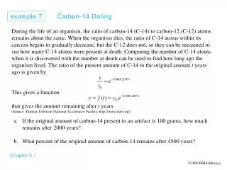
Use the option to rerun the job Now we will rerun the model using the Isentropic vertical motion option to demonstrate the differences observed between model vertical motion and Isentropic motion. Vertical Motion: Isentropic Vertical plot height units: Theta Click on “Rerun the model with user entered defaults” from the results page. Also, Uncheck “Plot meteorological field along trajectory” and uncheck “Mixed Layer Depth.”
Shown below left is the trajectory from Example 7 using the NAM 12 km vertical velocity fields. To the right is the same trajectory computed using the isentropic flow assumption and choosing the Theta vertical coordinate option. This graphic shows that the potential temperature varied by only about 1 degree, however by assuming adiabatic flow conditions the second trajectory ended in northeastern Louisiana after 84 hours instead of north central Texas. The validity of the adiabatic flow assumption would need to be assessed for this case (no precipitation, cloud, etc). Model Vertical Velocity Isentropic