Chapter 12 Coupled Oscillations
380 likes | 815 Views
Chapter 12 Coupled Oscillations. Claude A Pruneau Wayne State University. 12.1 Introduction Coupled equations Normal coordinates Normal modes n degrees of freedom (n-coupled 1-d oscillators or n/3-coupled 3-d oscillators) leads to n normal modes (in general)

Chapter 12 Coupled Oscillations
E N D
Presentation Transcript
Chapter 12Coupled Oscillations Claude A Pruneau Wayne State University
12.1 Introduction • Coupled equations • Normal coordinates • Normal modes • n degrees of freedom (n-coupled 1-d oscillators or n/3-coupled 3-d oscillators) leads to n normal modes (in general) • some of the modes may be identical.
12.2 Two coupled harmonic oscillators. • Example: In a solid, atoms interact by elastic forces and oscillate about their equilibrium positions. • Let’s consider the following simpler system m1=M m2=M 1= 12 2= x2 x1
Consider a solution of the form Frequency, , to be determined, and amplitudes may be complex.
A solution to these Eqs exist if the 2x2 determinant is null. This yields
There are two characteristic frequencies The general solution is thus
The amplitudes are not all independent given that they must satisfy. The solutions may thus be written:
There are four arbitrary constants - as expected given one has two equations of second order.
add subtract
1 f 0 2 1 2 = 0 0 3
X1(t) t X2(t) t
In general, we then find where By construction:
finite mij and Ajk express the coupling between the various coordinates.
We get A non trivial solution to this equation exists only if A secular Eq. of degree n in 2. Implies n roots for 2