Download
1 / 17
170 likes | 393 Views
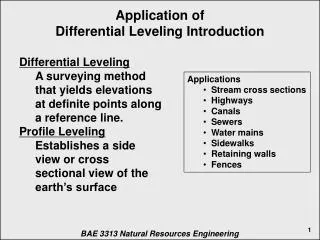
Application of Differential Leveling Introduction. Differential Leveling A surveying method that yields elevations at definite points along a reference line. Profile Leveling Establishes a side view or cross sectional view of the earth’s surface. Applications Stream c ross sections

E N D
Application of Differential Leveling Introduction • Differential Leveling • A surveying method that yields elevations at definite points along a reference line. • Profile Leveling • Establishes a side view or cross sectional view of the earth’s surface • Applications • Stream cross sections • Highways • Canals • Sewers • Water mains • Sidewalks • Retaining walls • Fences BAE 3313 Natural Resources Engineering
Characteristics Single segment Multiple segments with changes in direction Straight segments connected with curves
Procedure • Common practice to use a procedure called stationing • Stations are established at uniform distances along a route, e.g. 100 feet • Half or quarter stations are used when the topography is very variable. • The distance from the starting point to the station is used as the station identification.
Procedure - cont. • Foresights (FS) are recorded at each standard station • Intermediate foresights (IFS) • Additional stations as needed to accurately define the topography. • Foresights (FS) taken at stations that are not used as benchmarks (BM) or turning points (TP).
Procedure - cont. • When distances to foresights (FS) become too long or when the terrain obstructs the view of the instrument, turning points (TP) are established. • Profile leveling is differential leveling with the addition of intermediate foresights (IFS).
Profile Data Table STA Station BS Back Site HI Height of Instrument FS Foresight IFS Intermediate Foresight ELEV Elevation
ExampleDetermine the profile for a proposed sidewalkthat connects two existing sidewalks. Step One: establish standard stations Note: last station is established even though it is not a standard station.
Step 2: Determine sites for critical features • In this example, the critical features are the rapid change is slope at 337.5 ftand the road at 489.6 ft • Note: a station was established at 546.4 ftto define the width of the road and any changes in elevation across the road.
Step 3: Set up instrument; start collecting data • First rod reading is a backsight (BS) on the first sidewalk (i.e. benchmark, BM) to establish the height of the instrument. • Note: the true elevation of the benchmark (BM) is unknown, therefore 100.00 feet is used.
Example Data Table STA Station BS Back Site HI Height of Instrument FS Foresight IFS Intermediate Foresight ELEV Elevation HI = ELEV + BS ELEV = HI - FS
Step 4: Start recording the rod readings at each station. Note: this station is not used as a benchmark (BM) or as a turning point (TP), therefore it is an intermediate foresight (IFS).
Example Data Table STA Station BS Back Site HI Height of Instrument FS Foresight IFS Intermediate Foresight ELEV Elevation HI = ELEV + BS ELEV = HI - FS
Rod reading for each station is recorded on the appropriate table line. Note: rod reading for station 489.6ft is placed in the FS column because this station will be used as a turning point (TP).
Step 5: Instrument is moved so the remaining stations can be reached. Note: every time the instrument is moved, a backsight (BS) is used to reestablish the height of instrument (HI).
Plot of Profile Data In this example the steepest slope appears to be between stations 300 and 327.5. The slope at this point is: