Download
1 / 50
500 likes | 749 Views
OUR Ecological Footprint - 1. 6…. Ch 20 Community Ecology: Species Abundance + Diversity. Objectives. Species relative abundance Species diversity Measures to quantify and compare SD Species-area relationship Factors affecting local SD Regional influences

E N D
Objectives Species relative abundance Species diversity Measures to quantify and compare SD Species-area relationship Factors affecting local SD Regional influences Species sorting
Species in communities vary in relative abundance. Are most species rare or common? % quadrats occupied Figure 1
What is the likelihood of sampling a rare species? A common species? How accurate are the data for rare species?
Log scale… Species abundance (dominance diversity) curves…Which community has 1) most species? 2) most variation in relative abundances? Figure 2
***Which variables can be used to describe the species diversity of a local community? Which community is more diverse? Species richness Species relative abundance Figure 3
Measures of community structure Species richness: # of species BUT species differ in abundance and thus in role Species diversity: weight species by their relative abundance Shannon-Wiener index: H' = - pi ln pi
Calculate Species Diversity:Species No. Ind. pi pi2ln pi pi ln pi 1 5 .25 .0625 -1.386 -.3465 2 4 .20 .0400 -1.609 -.3218 3 3 .15 .0225 -1.897 -.2846 4 4 .20 .0400 -1.609 -.3218 5 4 .20 .0400 -1.609 -.3218Total (N) 20 1.00 ∑=.205∑= -1.5965 • H' = -∑pi ln pi = 1.5965
Comparisons of diversity indices among communities. C1 C2 C3 C4 C5 • Which community is most diverse? • What factors increase species diversity? • more species. • less difference in relative abundance • among species. Figure 4
What is the relationship between species # and area? What scales are used? log log Figure 5
Species - area relationship: S = c Az S = # of species A = area c and z = fitted constants log S= log c + z log A = linear z = slope of line
***Why do larger areas have more species? in part because… larger areas -->larger samples but also… greater habitat heterogeneity (sample more types of habitats) larger islands---> bigger target for immigrants larger populations ---> greater genetic diversity broader distributions over habitats less stochastic extinction
What contributes to these species-area relationships?. Figure 6
Slope (z) of species-area relationship: affected by different processes at different scales Local Regional World Figure 7
Multiple scales of species diversity • Local • Regional • Latitudinal • Continental • Global
Factors Affecting SD at Local Scale: • Abiotic factors • Biological interactions • Dispersal limitation • Human introduction • Chance
QUESTION: Abiotic factors + Diversity • A 100-yr experiment tested the effect of fertilizer on species diversity (H’) in a grassland. • RESULTS: H’ of unfertilized remained steady. • H’ of fertilized decreases through time. • Summarize the major result of the study. • What 2 components of a community does the Shannon-Wiener Index (H’) incorporate? • What combination of these components yields the greatest value of H’? • Explain the results in terms of competition and niche theory. Figure 8
Compare the relationship of climate variablesand species richness along latitude. Figure 9
Biotic Hypotheses to explain variation in species richness 1 Heterogeneity in space and time e.g. (Vegetation and food complexity) 2 Herbivore and pathogen pressure 3 Competition/niches Other hypotheses 4 Disturbance 5 Equilibrium models
1 Heterogeneity in space and time hypothesis Relates to niche arguments (see below)
Species richness increases as a stream becomes larger and has more habitat and food diversity.
2) Pest pressure (herbivores + pathogens) hypothesis for maintaining tree species richness Figure 10
Distance-dependent (+/or) density-dependent) mortality is consistent with the pest pressure hypothesis. Figure 11
Summarize two results relating to how pathogens could enhance species richness. Figure 12
3 Competition hypothesis: • High richness --> less competitive exclusion?--> more species • Why? By what means?
How can more species be added to a community? • Increase total niche space • Increase niche overlap • Decrease niche breadth Figure 13
4 Competition hypothesis, cont.: • High richness --> less competitive exclusion? • Why? By what means? • greater specialization (narrower niche) • greater resource availability (greater niche space); less niche overlap • reduced resource demand (smaller populations) • Greater niche space from greater number of niche axes and length of each axis? • relates to hypothesis of heterogeneity in space/time
Does increase in niche diversity --> increase in species richness? As s.r. increases, so does morphological diversity.
Populations in regions with few species show ecological release (and larger realized niches).
Realized niche is always smaller than fundamental niche, • but with ecological release ---> larger realized niches
4 Intermediate Disturbance Hypothesis • Richness peaks at intermediate levels • Too low disturbance --> competitive exclusion • Too high disturbance --> limited number of species adapted
5 Equilibrium hypothesis • Richness reaches an equilibrium when factors • removing species = factors adding species. • What process adds species? • What process removes them? • more additions (e.g. speciation) or and/or fewer deletions (e.g. extinctions) = greater species richness.
Hubbell’s Neutral Model of Random Drift Species competitively equivalent (neutral) Pests + recruitment limitation reduce comp. Limited ecological specialization Stochastic processes of B and D --> reduce community to 1 species Species richness depends on speciation and immigration Figure 14
Multiple scales of species diversity • Local • Local Affected by Regional • Regional • Latitudinal • Continental • Global
Species richness (# species) has both local and regional components. (alpha) = local # species in small area of homogeneous habitat (beta) = # species turnover between habitats (gamma) = (landscape) regional: total # species in all habitats within a barrier-free geographic area
Above species richness measures determined by ecology and regional pool (delta) = available pool of species within dispersal distance (up to continental scale) determined evolutionarily
What are two patterns of species turnover (beta diversity) at larger scales? Figure 16
What is the major change in longitudinal beta diversity with increasing latitude?Which latitude has more climatic uniformity? Figure 17
Regional diversity sets limit on local diversity.Local then determined by many factors. Figure 18
Local communities contain a subset of the regional species pool. • ***What determines whether a species can be a member of a given community? 1 Adaptations of species to environmental conditions (habitat selection) 2 Persistence in face of competitors, predators, and parasites 3 Stochastic extinction
Local communities are assembled from the regional species pool. • Species sorting = processes that determine local community composition.
Experimentally-composed communities show species sorting. What caused the sorting? Regional: # species available Fertility: low high Local: realized # Figure 19
Environmental filters eliminate species thatcan’t tolerate conditions---> species sorting Figure 20
What is the major and minor factor sorting species in this community? Figure 21
H1:Species sorting should be greatest where regional species pool is largest. • When species pool is smaller, competition should be relaxed---> • ecological release= species expand into habitats normally filled by other species and increase in population density • Ecological release provides evidence for hypothesis of local interactions controlling species diversity. • (e.g. competition for resources structures communities and limits # species)