Inferential Statistics

1. Inferential Statistics Confidence Intervals and Hypothesis Testing

2. Samples vs. Populations • Population • All of the objects that belong to a class (e.g. all Darl projectile points, all Americans, all pollen grains) • A theoretical distribution • Sample • Some of the objects in a class • Observations drawn from a distribution

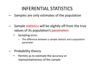
3. Two Distributions • The sample distribution is the distribution of the values of a sample – exactly what we get plotting a histogram or a kernel density plot • The sampling distribution is the distribution of a statistic that we have computed from the sample (e.g. a mean)

5. Confidence Intervals • Given a sample statistic estimating a population parameter, what is the parameter’s actual value? • Standard Error of the Estimate provides the standard deviation for the sample statistic:

6. Example 1 • Snodgrass house size. Mean area is 236.8 with a standard deviation of 94.25 based on 91 houses. • Area is slightly asymmetrical • Can we use these data to predict house sizes at other Mississippian sites?

8. Example 1 (cont) • The confidence interval is based on the mean, sd, and sample size • Mean ± t(p<confidence)*sd/sqrt(n) • For 95% , 90%, 67% confidence • qt(c(.025,.975), df=90) • qt(c(.025,.975), df=90) • qt(c(.167,.833), df=90)

9. # Distributions x <- seq(10, 40, length.out=200) y1 <- dnorm(x, mean=25, sd=4) y2 <- dnorm(x, mean=25, sd=1) max(y2) plot(x, y1, type="l", ylim=c(0, .4), col="red") lines(x, y2, col="blue") text(c(28, 26.3), c(.08, .30), c("Sample Distribution\n mean=25, sd=4", "Sampling Distribution\n m=25, sd=1, n=16)"), col=c("red", "blue"), pos=4) # Snodgrass House Areas plot(density(Snodgrass$Area), main="Snodgrass House Areas") lines(seq(0, 475, length.out=100), dnorm(seq(0, 475, length.out=100), mean=236.8, sd=94.2), lty=2) abline(v=mean(Snodgrass$Area)) legend("topright", c("Kernel Density", "Normal Distribution"), lty=c(1, 2)) # Confidence interval function conf <- function(x, conf) { conf <- ifelse(conf>1, conf/100, conf) tail <- (1-conf)/2 mean(x)+qt(c(tail, 1-tail), df=length(x)-1)*sd(x)/sqrt(length(x)) }

10. Bootstrapping • Confidence intervals depend on a normal sampling distribution • This will generally be a reasonable assumption if the sample size is moderately large • We can draw multiple samples of house areas to get some idea

12. # Draw 100 samples of size 50 samples <- sapply(1:100, function(x) mean(sample(Snodgrass$Area, 50, replace=TRUE))) range(samples) quantile(samples, probs=c(.025, .975)) conf(Snodgrass$Area, 95) plot(density(samples), main="Sample Size = 50") x <- seq(175, 300, 1) lines(x, dnorm(x, mean=mean(samples), sd=sd(samples)), lty=2) legend("topright", c("Kernel Density", "Normal Distribution"), lty=c(1, 2)) # Draw 1000 samples of size 91 samples <- sapply(1:100, function(x) mean(sample(Snodgrass$Area, 91, replace=TRUE))) range(samples) quantile(samples, probs=c(.025, .975)) conf(Snodgrass$Area, 95) plot(density(samples), main="Sample Size = 91") x <- seq(175, 300, 1) lines(x, dnorm(x, mean=mean(samples), sd=sd(samples)), lty=2) legend("topright", c("Kernel Density", "Normal Distribution"), lty=c(1, 2))

13. Example 2 • Radiocarbon Ages are presented as an age estimate and a standard error: 2810 ± 110 B.P. • The probability that the true age is between 2700 and 2920 B.P. is .6826 or .3174 that it is outside that range • The probability that the true age is between 2590 and 3030 B.P. is .9546 or .0545 that it is outside that range

14. Hypothesis Testing • Assumptions and Null Hypothesis • Test Statistic (method) • Significance Level • Observe Data • Compute Test Statistic • Make Decision

15. Assumptions • Data are a random sample • Every combination is equally likely • Appropriate sampling distribution

16. Null Hypothesis • Represented by H0 • Must be specific, e.g. S1-S2 = 0 • The difference between two sample statistics is zero, e.g. they are drawn from the same population (two tailed test) • Or S1-S2>0 (one tailed)

17. Test Statistic • Measurement Levels • Number of groups • Dependent vs. Independent • Power

18. Significance Level • Nothing is absolute in probability • Select probability of making certain kinds of errors • Cannot minimize both kinds of errors • Social scientists often use p ≤ 0.05 • Consider how many tests

19. Errors in Hypothesis Testing

20. Difference of Means (t-test) • Independent random samples of normally distributed variates • Samples: 1, 2 independent, 2 related • If 2 independent – variances equal or unequal • Sample statistics follow the t-distribution

21. Example • Snodgrass site is a Mississippian site in Missouri that was occupied about A.D. 1164

23. Using Rcmdr • Snodgrass Site – House sizes inside and outside are the same • Check normality - shapiro.test() • Check equal variances – var.test() or bartlett.test() • Compute statistic and make decision – t.test()

24. Wilcoxon Test • If data do not follow a normal distribution or are ranks not interval/ratio scale • Nonparametric test that is similar to the t-test but not as powerful • Tests for equality of medians • wilcox.test()

25. Difference of Proportions • Uses the normal distribution to approximate the binomial distribution to test differences between proportions (probabilities) • This approximation is accurate as long as N x (min(p,(1-p))>5 where N is the sample size, p is the proportion, and min() is the minimum

26. Using Rcmdr • Must have two or more variables defined as factors, eg, • Create ProjPts to be equal to as.factor(ifelse(Points>0, 1, 0)) using Data | Manage variables . . . | Compute new variable • Statistics | Proportions | Two sample . . . • prop.test() • Are the % Absent equal inside and outside the wall?