Understanding Matching Techniques in Causal Studies: A Comprehensive Overview
This summary explores matching techniques used in causal studies, focusing on the importance of finding control units to match treated groups. Key topics include one-sided versus two-sided p-values, the concept of imputation for missing treatment outcomes, and methods such as exact matching, inexact matches, and matching with replacement. The content emphasizes the significance of covariate balance, bias adjustment, and tackling multiple covariates through distance metrics. Practical insights on matching strategies, including greedy and hybrid matching approaches, are also discussed to aid researchers in estimating treatment effects effectively.

Understanding Matching Techniques in Causal Studies: A Comprehensive Overview
E N D
Presentation Transcript
Matching STA 320 Design and Analysis of Causal Studies Dr. Kari Lock Morgan and Dr. Fan Li Department of Statistical Science Duke University
Quiz 2 > summary(Quiz2) Min. 1st Qu. Median Mean 3rd Qu. Max. 11.0 14.0 15.0 15.5 17.0 20.0
Quiz 2 • one-sided or two-sided p-value? (depends on question being asked) • imputation: use observed control outcomes to impute missing treatment outcomes and vice versa. • class year: use observed outcomes from control sophomores to impute missing outcomes for treatment sophomores • biased or unbiased
Matching • Matching: Find control units to “match” the units in the treatment group • Restrict the sample to matched units • Analyze the difference for each match (analyze as matched pair experiment) • Useful when one group (usually the control) is much larger than the other
Estimand • Changes the estimand: now estimating the causal effect for the subpopulation of treated units • ATE: Average treatment effect • ATT: Average treatment effect for the treated • ATC: Average treatment effect for the controls
Exact Matching • For exact matching, covariate values must match exactly • 21 year old female in treatment group must be matched with 21 year old female in control group
Inexact Matches • Often, exact matching is not feasible, and matches are just as close as possible • The farther apart the matches are, the more bias there will be • Bias: covariate imbalance • There are ways of adjusting for bias (ch 18) • Can use calipers: only matches within a certain caliper are acceptable (remove units without an acceptable match)
Matching uh oh…
Ideal Matches • Ideal: minimize total (or average) covariate distance for pairs • Hard to do computationally, especially for large sample sizes
“Greedy” Matching • Greedy matching orders the treated units, and then sequentially chooses the closest control (ignoring effect on later matches) • When doing this, helps to first match units that will be hardest to match • One possibility: order by decreasing propensity score (treated units with highest propensity scores are most unlike controls)
Matching with Replacement • Matching can be done with replacement • Pros: • Easier computationally (ideal matches overall same as just closest for each unit) • Better matches • Cons: • Variance of estimator higher (controls can be used more than once, so less information) • Variance is harder to estimate (no longer independent)
Matching with Replacement • Matching with replacement is necessary if the group you want to make inferences about is the smaller group • Matching with replacement also allows you to make inferences about the entire sample (find a match for every unit, from opposite group) • Units more similar to those in the opposite group will be selected more
Multiple Covariates • With multiple covariates, how do you know which to prioritize? • 21 year old female • Which is a better match: • 18 year old female • 21 year old male • Want a way to measure multivariate covariate distance
Distance Metric • Lots of different possible distance metrics • Mahalanobisdistance? • Sum of squared (standardized) covariate difference in means? • Difference in propensity scores? • Linearized propensity score…
Linearized Propensity Score • Difference between propensity scores of 0.001 and 0.01 is larger than difference between propensity scores 0.1 and 0.109 • Better option: linearized propensity score, the log odds of propensity score: • Logistic regression:
Linearized Propensity Score • Note: the linearized propensity score is recommended for subclassification as well, although it isn’t as important in that setting • Won’t change subclasses, but will change your view of whether a subclass is small enough
Hybrid Matching • In hybrid matching, match on more than one criteria • Example: exact matches are required for some covariates, and other covariates are just as close as possible • Example: 21 year old female; look for closest age only within female controls • Example: match on propensity score and important covariate(s)
Multiple Matches • Paired matching is called 1:1 matching (1 control to 1 treated) • If the control group is much bigger than the treatment group, can do 2:1 matching (2 controls to 1 treatment unit), or more to one matching • Another option: caliper matching in which all controls within a certain distance (based on some metric) of a treated unit are matched with that unit
Matching • Like propensity score estimation… • and like subclassification…. • … there are no “right” matches • If the matches you choose give good covariate balance, then you did a good job!
Decisions • Estimating propensity score: • What variables to include? • How many units to trim, if any? • Subclassification: • How many subclasses and where to break? • Matching: • with or without replacement? • 1:1, 2:1, … ? • how to weight variables / distance measure? • exact matching for any variable(s)? • calipers for which a match is “acceptable”? • …
Lalonde Data • Analyze the causal effect of a job training program on wages • Data on 185 treated (participated in job training program) and 2490 controls (did not participate in job training program) • GOAL: achieve covariate balance!
To Do • Read Ch 15, 18 • Homework 4 (due Monday)