Download
1 / 27
270 likes | 437 Views
The ATLAS Insertable B-Layer (IBL) Project C. Gemme, INFN Genova On behalf of the ATLAS IBL COllaboration. RD11 Firenze - 6-8 July 2011. ATLAS Pixel Detector: Layout. Designed to provide at least 3 hits in | h | < 2.5 3 barrel +3 forward/backward disks

E N D
The ATLAS Insertable B-Layer (IBL) Project C. Gemme, INFN Genova On behalfof the ATLAS IBL COllaboration RD11 Firenze - 6-8 July 2011
ATLAS Pixel Detector: Layout • Designed to provide at least 3 hits in |h| < 2.5 • 3 barrel +3 forward/backward disks • 112 staves with 13 modules each • 48 sectors with 6 modules each • 80 million channels • ~0.11 X0 Talk by D.Hirschbuehl
ATLAS Pixel Detector: Module • The building block of the detector is the module (1744 in total). • 16 Front-End chips (FE-I3) with a module controller (MCC), 0.25 mm technology. • 46080 R/O channels 50mmx400mm • Planar n-in-n DOFZ silicon sensor 250 mm thick. • Readout speed 40-80 Mb/link • Designed for NIEL 1x10¹⁵neq/cm2, 50 Mrad dose and a peak luminosity of 1x1034 cm-2s-1 • Foreseen to replace the Pixel detector in ~2021 (HL-LHC). Talk by D.Hirschbuehl Dimensions: ~ 2 x 6.3 cm2 Weight: ~ 2.2 g
Insertable B-Layer: Project • The Pixel innermost layer (B-layer) was designed for replacement every 300 fb-1 • the requirements for replacibility in a long shutdown were released in the building phase. • New option (Feb 2009): to insert a new layer! • The envelopes of the existing Pixel detector and the beam pipe leave today a radial free space of 8.5 mm. The reduction of the beam-pipe radius of 5.5 mm brings it to 14 mm and make it possible. • The Insertable B-Layer IBL will be built around a new beam pipe and slipped inside the present detector in situ. O(9 months) needed. Existing B-Layer First Pixel Upgrade!
Insertable B-Layer: Layout • Reduced Beam Pipe • Inner Radius 23.5 mm. • Very tight clearance • Hermetic to straight tracks inf • No overlap in z: minimum gap between sensor active area! • Layout parameters: • IBL envelope : 9 mm in R! • 14 staves • <Rsens> = 33 mm • Total active length = 60 cm • Coverage in |h| < 2.5
Insertable B-Layer: Motivations • Motivations for a 4th low radius layer in the Pixel Detector • Luminosity pileup • FE-I3 has 5% inefficiency at the B-layer occupancy for 2.2x1034cm-2s-1 • IBL improves tracking, vertexing and b-tagging for high pileup and recovers eventual failures in present Pixel detector. • Today the B-layer has 3.1% of inefficiency. • Radiation damage • Degradation of the existing B-Layer reduce detector efficiency after 300-400 fb-1. Not an issue as forecast for 2021 is ~ 330 fb-1 • It serves also as a technology step towards HL-LHC. • IBL Installation foreseen in 2013, during LHC first shutdown. Occupancy B-Layer 2x1034 1x1034
Insertable B-Layer: Performance • b-tagging performance with IBL at 2x1034 cm-2s-1 is similar to current ATLAS without pileup • Studied scenarios with detector defects, the IBL recovers the tracking and b-tagging performance. • Shown 10% cluster inefficiency in B-layer. • IBL fully recovers tracking efficiency. • With IBL only small effect on b-tagging performance +IBL ATLAS 1x1034 2x1034 +IBL ATLAS
Requirements for sensors/electronics • IBL environment: Radiation hard FE and sensor. • Integrated luminosity seen by IBL = 550 fb-1 Survive until to HL-LHC • IBL design peak luminosity = 3x1034 cm-2s-1 • Design sensor/electronics for total dose: • NIEL dose = 3.3 x 10¹⁵ ± (“safety factors”) ≥ 5 x 10¹⁵ neq/cm2 • Ionizing dose ≥ 250 Mrad • Two different pixel sensor technologies will be used: • n-in-n planar and 3D silicon detectors. • Extra specifications: • Sensor HV: max 1000 V • Sensor Thickness: 225±25µm. • Sensor Edge width: below 450 µm (No shingling in z ) • Tracking efficiency > 97% • Sensor max power dissipation < 200 mW/cm2at T = -15 0C • Operation with low (~1500e-) threshold. X 5 the Pixel detector
FE electronics • Reason for a new FE design: • Increase rad hardness • Reduce inefficiency at high luminosity • New logic: instead of moving all the hits in EOC (FE-I3), store the hits locally in each pixel and distribute the trigger. • Advantages: • Only 0.25% of pixel hits are shipped to EoC DC bus traffic “low”. • Save digital power • Take higher trigger rate • At 3×LHC full lumi, inefficiency: ~0.6% • This requires local storage and processing in the pixel array • Possible with smaller feature size technology (130 nm) • Biggest chip in HEP to date: 4 cm2
Dose and noise • Typical noise of the bare FE after calibration ~ 110e-. Measured before and after irradiation for different DAC settings. • 800 MeV proton irradiation at Los Alamos: • 6 / 75 / 200 MRad. calib ~×1.15 Ratio noise after / before dose
Low threshold operation • Studies on PPS and 3D assemblies irradiated with protons to 5 1015neq/cm2. • Noise occupancy increase when Threshold below 1500e-. • At 1100 e-, occupancy is ~10-7 hits/BC/pixel. • Low threshold operation with irradiated sensors demonstrated! Masked pixel floor = digitally un-responsive pixels. 10-7
2-Chip Planar Sensor • Main advantage: • All benefits of a mature technology (yield, cost, experience). • Main challenges: • Low Q collection after irrad, • Low threshold FE-operation. • High HV needed: important requirement for the services and cooling. • Inactive area at sensor edge. • Slim edge sensors. Wafer at CiS, Germany IV@-15 °C
2-Chip Planar Sensor: Performance • Final choice for the IBL design: • Thickness is 200 um. Best compromise between Charge collection and material budget. • n-in-n technology with ~200 μm slim edge (is 1100 um in the Pixel detector) • Slim edge: 500 μm long edge pixels with guard ring shifted underneath on the opposite side from pixel implant. • Only moderate deterioration. 250/200 um of inactive edge before/after irradiation. Bring to total geometrical inefficiency of 98.3-98.5%. • High efficiency (>97%) for tracks at operation conditions (see next slide). 1000V, n=3.7E15, Φ=15 o
2-Chip Planar Sensor: Performance 1000V, n=3.7E15, Φ=15 o
1-Chip 3D Sensor • Main advantage: • Radiation hardness. • Low depletion voltage (<180V). • Main challenges: • Production yield. • In-column inefficiency at normal incidence. • Active edges and full 3D processing not established enough on project time scale. • Two vendors CNM and FBK • Production schedule requires aggregate production Wafer at CNM Spain / FBK Italy FE-I4 SC FE-I4 SC FE-I4 SC FE-I4 SC FE-I4 SC FE-I4 SC FE-I4 SC FE-I4 SC
1-Chip 3D Sensor • Main advantage: • Radiation hardness. • Low depletion voltage (<180V). • Main challenges: • Production yield. • In-column inefficiency at normal incidence. • Active edges and full 3D processing not established enough on project time scale. • Two vendors CNM and FBK • Production schedule requires aggregate production. • Double-Sided full passing 3D, 2 electrodes per pixel • ~10 µm column diameter • ~ 70 µm interdistance • Wafer yield ~ 55% 700nm DRIE stopping membrane FBK DRIE: Full thru columns
1-Chip 3D Sensor: Performance Leakage currents for CNM and FBK Am source scan Voltage and currents vs fluence
1-Chip 3D Sensor: Efficiency p-type Bias Electrodes n-type read-out Electrodes SCC97: CNM, p-5E15, Φ=15 o SCC87:FBK, p-5E15, Φ=15 o SCC82: CNM, n-5E15, Φ=15 o Test Beam Analysis On-going Efficiency >95% but need to Measure with lower threshold.
1-Chip 3D Sensor: Edge Efficiency • For 3D sensor the edge pixel has a regular length. • Inactive area: 200 μm • Actual efficiency extends: • 50%: 20-30 μm • Effective inactive area from dicing: ~200 μm. • Same for all 3D samples. 200μm 250μm
Sensor choice • Sensor Review hold on July 4/5. Fresh News! • The review panel found nothing is wrong in the 2 technologies. • Proposed a mixed scenario with both sensors in: • 3D technology to populate the forward region where the tracking could take advantage of the electrode orientation to give a better z-resolution after heavy irradiation • Target to 25% coverage with 3D – Verify in February 12 where we stand then move up to 50%. • Anyhow Continue the production of the Planar to cover the whole IBL. 3D at 25% 3D at 50% Stave = 32 FEs divided in 8 group of 4 FEs each that share LV and HV. Do not want to mix sensors in a group.
Modules • IBL modules preproduction with Planar and 3D sensors • Over 78 single-chip assemblies produced for the sensor qualification. • Many of those irradiated to check design requirements. • Bump bonding yield at IZM around 85%. Good for the start-up with FEI4. • Now addressing thinner electronics • Thin (100-150 mm) FEI4 for a low X0 module. • Safe bump-bonding requires max bend of ~15µm. Achievable with a minimal thickness of 450µm. Use temporary glass handling wafer + laser de-bonding. • First devices produced and under tests. • Module flex on top for final assembly • Up to now just used test card. SingleChipCard
Stave • Mechanical structure: • Tested a large number of prototypes to find right balance between thermal performance, mechanical stiffness and reasonable X0. • Shell structure filled with light (0.2g/cc) carbon foam for heat transfer to central cooling pipe (1.5mm ID Ti pipe 0.1mm thick) • Cooled with CO2 system at -40C (~1.5kW total). • Services on the back • 500 mm Flex Al/Cu bus glued/laminated on the stave backside to route signals and power lines. (Al-only solution in parallel) • The flex design include wings to be folded and glued to the modules. 53 cm
Conclusions • Tight schedule for installation in 2013 shutdown. On the critical path: • New revision of the FEI4 submitted in July and back in October. • Bump bonding with thin electronics. • Keep the material under control (1.5% X0)
Charge collection Planar • Charge collection Am in 3D C. Gemme, INFN Genova, LPP
Off-detector FEI4 powering • FE-I4 voltage regulators proposed to be set in partial shunt mode to guarantee a minimal current. The goal is to limit transient voltage excursion. • First complete prototype of optobox in October • ROD fabrication has started: 2 prototypes expected by next month • ROD firmware design is ongoing • The design of a full DAQ chain simulation environment has started • BOC: prototypes expected by September, then testing and redesign until the end of the year • RX plugin: investigation underway to use commercial SNAP12 modules • Grounding & Shielding concept is now integrated into the whole IBL detector BOC block diagram Optobox concept for nSQP and IBL 27