Download
1 / 40
420 likes | 784 Views
Chapter 12 Electing the President. Paul Moore. Presentation Outline. What math can tell us about elections and strategy behind them Spatial Models (Candidate positions on issues) 2 candidates ( Unimodal , Bimodal) 2+ candidates (1/3 separation, 2/3 opportunity) Election Reform

E N D
Chapter 12Electing the President Paul Moore
Presentation Outline • What math can tell us about elections and strategy behind them • Spatial Models (Candidate positions on issues) • 2 candidates (Unimodal, Bimodal) • 2+ candidates (1/3 separation, 2/3 opportunity) • Election Reform • Approval Voting • Electoral College • Strategies to maximize: • Popular Votes • Electoral Votes
Running for President • Elections every 4 years • 35 years old • Native born citizens • US residents for 14 years • No third term
How to become President • Democratic and Republican Primaries • Candidates campaign for party nomination • Party nominates candidates • National conventions • General Election • 2-3 serious contenders • Electoral College
Math & Presidential Elections • Campaign strategies • Choosing states to campaign based on electoral college weight • Effects of reform on these strategies • Approval voting • Popular voting (without Electoral College) • Candidates getting a leg up in the primaries to help them win their party’s nomination • Spatial Models
Spatial Model: 2 Candidates • Model Assumptions: • Voters respond to positions on issues • Single overriding issue, candidates must chose side • Voter attitudes represented as “left-right continuum” (very liberal to very conservative) • Unimodalvs Bimodal • Voter distribution represented by curve, giving number of voters with attitudes at different points on L-R continuum
Unimodal Distribution Number of voters Candidate A M Candidate B Voter Positions on L-R Continuum • Unimodal – one peak, or mode • Pictured as continuous for simplicity • Median, M– of a voter distribution is the point on the horizontal axis where half the voters have attitudes that lie to the left, and half to right
Unimodal Distribution Number of voters Number of voters Candidate A Candidate B Candidate A Candidate B M M Voter Positions on L-R Continuum Voter Positions on L-R Continuum • Attitudes are a fixed quantity, decisions of voters depend on position of candidates • Candidate positions: Candidate A (yellow line), Candidate B (blue line) • Assume voters vote for candidate with attitudes closest to their own (and that all voters vote) • What happens in models above?
Unimodal Distribution • “A” attracts all voters to the left of M, while “B” attracts all voters to the right of M • Any voters on the horizontal distribution between “A” and “B” (when they are not side by side) are split down the middle Number of voters Candidate A Candidate B M
Unimodal Distribution • Maximin – the position for a candidate at which there is no other position that can guarantee a better outcome (more voters), no matter what the other candidate does • At what position is a candidate in maximin? • Is there more than one maximin position? • Taking position at M guarantees a candidate 50% of the votes, no matter what the other candidate does • Is there any other position that can guarantee a candidate more? • No, there is no other position guaranteeing more votes
Unimodal Distribution • Further more M is stable, meaning that once a candidate chooses this position, the other candidate has no incentive to choose any other position except M. • M is a maximin for both candidates, and they are in equilibrium • Equilibrium – when a pair of positions, once chosen by candidates, does not offer any incentive to either candidate to depart from it unilaterally • Is there another equilibrium position(s)?
Unimodal Distribution • Equilibrium Positions…unique? • 2 cases: • Common point – both candidates take the same position • Distinct positions – one taken by each • Case 1: Common Point • If candidates are in at a common point, to the left of M for example, then one candidate can always do better by moving right but staying on the left of M. The same idea can be applied to common points to the right of M. So common position other than M cannot be equilibrium • Case 2: Distinct Positions • If candidates are in two different positions then one candidate may always do better by moving alongside of the other candidate, gathering more voters. So distinct positions cannot be in equilibrium.
Unimodal Distribution • …From this we get the Median Voter theorem • Median Voter Theorem – in 2 candidate elections with an odd number of voters, M is the unique equilibrium position • Bimodal distribution?
Bimodal Distribution Number of voters • Use same logic as unimodal distribution to examine unique equilibriums • Again at M, a candidate is guaranteed at least 50% of the votes no matter what the other candidate does • It is a maximin for both candidates, and an equilibrium • Any others? M
Bimodal Distribution Number of voters • 2 Cases for possible equilibriums (other than M) • Common point – both candidates take the same position • Distinct positions – one taken by each • Case 1: Common Point • If candidates are in at a common point, to the left of M for example, then one candidate can always do better by moving right but staying on the left of M. The same idea can be applied to common points to the right of M. So common position other than M cannot be equilibrium • Case 2: Distinct Positions • If candidates are in two different positions then one candidate may always do better by moving alongside of the other candidate, gathering more voters. So distinct positions cannot be in equilibrium. M
Bimodal Distribution Number of voters • So using the same logic, we can see that M is the unique equilibrium for bimodal distributions (Median voter theorem) • Extension: • Median Voter Theorem can be applied to any distribution of electorate’s attitudes • This is because the logic for the proof does not rely on any modal characteristics. Only the idea that to the left and right of the median lies an equal distribution of voter attitudes M
Bimodal Distribution • How does M compare with the mean of the distribution • Mean of Voter Distribution where : n = total number of voters = n1+n2+n3+…+nk k = number of different positions i that voters take on continuum ni = number of voters at position i li = location of position i on continuum Σ is from i = 1 to k • Weighted average – location of each position is weighted by number of voters at that position • Exercise 1!
Bimodal Distribution • Exercise 1: • Mean need not coincide with median M • In exercise, distribution is skewed to the left • Area under the curve is less concentrated to the left of M than to the right • From Median Voter Theorem: • if the distribution is skewed, then it may not be rational for candidates to choose the mean of the distribution • Even number of voters? • Equilibrium positions? • Median: 0.6, Mean: 0.56
Bimodal Distribution • Even # of Voters, Discrete Distribution • Discrete Distribution of voters - where voters are located at only certain positions along the left-right continuum (like in the exercise) • Consider example: • n = 26 • k = 8 different positions over interval [0, 1] • Mean = 0.5 • Median = 0.45 (average of 0.4 and 0.5)
Bimodal Distribution • Mean = 0.5 • Median = 0.45 (average of 0.4 and 0.5)
Bimodal Distribution • Both candidates at M, they’re in equilibrium • Is this equilibrium position still unique? • Any pair of positions between 0.4 and 0.5 is in equilibrium • Following that, distinct positions 0.4 and 0.5 are also in equilibrium • In general • With even number of voters and 2 middle voters have different positions then the candidates can choose those 2 positions, or any in between, and be in equilibrium M Mean = 0.5 Median = 0.45
Spatial Models: +2 Candidates • Primary elections often have more than 2 candidates • Under what conditions is a multicandidate race “attractive”? • Using a similar model, will examine the different positions of an entering 3rd candidate • Consider the unimodal 2 candidate race with both at M Is it rational for a 3rd candidate to enter the race? (are there any positions offering the candidate a chance at success?) Number of voters Candidate A (red) Candidate B (blue) M
Spatial Models: +2 Candidates Candidate A (red) Midway between A/B and C Number of voters • Candidate C enters race at position C on graph • C’s area of voters is yellow • A and B have to split the light blue voters • C wins plurality of votes Candidate B (blue) Candidate C (pink) M C A/B • Upon entry C gains support of voters to the right, and some to left • Blue votes are split between A and B, and C is left with the majority • C can also enter on the left side of M, still winning by the same logic • Can a 4th candidate, D, enter the race and win?
Spatial Models: +2 Candidates • Median M no longer appealing to candidates • Vulnerable • However, a 3rd candidate C will not necessarily win against both A and B • 1/3-Separation Obstacle • If A and B are distinct positions equidistant from M of symmetric distribution, and separated from each other by at most 1/3 of total area, then C can take no position that will displace A and B and enable C to win A B M
Spatial Models: +2 Candidates • 2/3 Separation Opportunity • If A and B are distinct positions equidistant from M on a symmetric distribution and separated by at least 2/3 of the area, then C can defeat both candidates by taking position at M A B M
Spatial Models: +2 Candidates • Not exactly to scale 1/6 each M A B 2/3 1/6 1/6
Spatial Models: +2 Candidates • Exercise 2 C C A B A B M M
Election Reform • Abolition of the Electoral College • More accurate and reliable ballots • Eliminating election irregularities • Most reforms ignore problem with multicandidate elections • Candidate who wins is not always a Condorcet winner • Approval Voting
Election Reform • Approval Voting • Voters can vote for as many candidates as they like or find acceptable. Candidate with the most approval votes wins. • 2000 Election • Came down to the “toss-up” state of Florida, where Bush won the electoral votes by beating Gore by a little over 300 popular votes • According to polls, Gore was the second choice of most Nader voters • In an approval voting system Gore would have almost certainly won the election since Nader supporters could have also given a vote of approval to Al Gore
Electoral College • Original purpose was to place the selection of a president in the hands of a body that, while its members would be chosen by the people, would be sufficiently removed from them so that it could make more deliberative choices. • How it works • Each state gets 2 electoral votes (for the 2 senators) • Also receives 1 additional electoral vote for each of its representatives in the House of Representatives (number of members for each state based on population) • Ranges from 1 in the smallest states to 53 in California • Altogether there are 538 electoral votes, so candidate needs 270 to win • In 2000, Bush received 271
Electoral College • Advantages in small states? • Technically California voters are about three times more powerful as individuals than those in the smallest states • Though in smallest states with 1 representative and 2 senators (3 electoral votes), the population receives a 200% (2/1) boost from having 2 senatorial electoral votes automatically. • California receives less than 4% (2/53) boost from senatorial electoral votes • Now that we know how it works, let’s examine it’s role in the 2000 election • Look at it as a game between 2 major party candidates • Develop 2 models • Candidates seek to max their expected popular vote • Candidates seek to max their expected electoral vote
Maximizing Popular Vote • Both models use the assumption that the probability of a voter in a “toss up state” ivotes for the Democratic candidate is: • where di and ri represent the proportion of campaign resources spent in state i by the Democratic and Republican candidates, respectively • The probability of a voter voting Republican is 1 – pi • Expected Popular Vote (EPV) • Is toss up states, the EPV of the Democratic candidate (EPVD) is the number of voters, ni, in toss up state i, multiplied by the probability, pi, that a voter in this toss up state votes Democrat, summed up across all toss up states is Basically a weighted average, weighted by probabilities
Electoral College • Candidates allocate resources across toss up states and attempt to do so in an optimal fashion • Democratic candidate seeks strategy di to maximize EPVD • Much like profit maximization among feasibility regions in Chapter 4 • Here some of the constraints are amount of campaign resources, time • Proportional Rule • Strategy of Democratic candidate to maximize EPVD, given Republican candidate also chooses maximizing strategy is: • Summed up across toss up states • Candidate allocates resources in proportion to the size of each state (ni/N) • Exercise 3
Maximizing Popular VoteCollege • The optimal spending strategy for each state (from di*and ri*) is • ($14M : $21M : $28M) on states 2, 3, and 4 respectively • Meaning the probability that either candidate will win any state i is 50% • pi= 50% for all itoss up states • So at optimal strategy, the EPV is the same for both candidates (D = R) • EPVDorR = 2[14/(14+14)] + 3[21/(21+21)] + 4[28/(28 + 28)] • Strategy sound familiar? • Candidates are at equilibrium • Now Exercise…what happens when departing from equilibrium?
Maximizing Popular Vote • Exercise 3 • Calculating p for the Republican candidate in 3 states • p1 = 14/14 • p2= 21/(21+27) • p3 = 28/(28+36) • EPVR • EPVR= 2[14/14] + 3[21/(21+27)] + 4[28/(28 + 36)] = 5.06 votes • or 56% of the 9 votes in those 3 states • Can the Republican candidate do even better? • Change his spending to ($2M : $26M : $35M) to achieve an • EPVR = 5.44 votes • *Departure from popular-vote maximizing strategy lowers candidates expected popular vote* Way to Go!!
Maxing Electoral Votes • Assume now goal is to max electoral votes • Candidate may think of throwing all resources into 11 largest states • 11 largest states have majority of electoral voters (271) • However, opponent may simply spend enough in 1 big state to defeat and use rest to spend small amounts in other 39, winning them • Expected Electoral Votes (EEV) • Where vi = number of electoral votes of toss-up state Pi = probability that the Democrat wins more than 50% of popular votes in state i
Maxing Electoral Votes • Expected Electoral Votes (EEV) • Calculating Pi • Must determine all probabilities that majority of voters in i will vote Democratic • 3 states: A, B, C with 2, 3, 4 electoral votes • Again, assume number of pop votes = number of electoral votes • State A: both voters • PA = (pA)(pA)) = (pA)2 • State B: 2 of 3 (3 ways) or all • PB = 3[(pB)2(1 – pB)] + (pB)3 • State C: 3 of 4 (4 ways) or all 4 • PC = 4[(pC)3(1 – pC)] + (pC)4
Maxing Electoral Votes • Strategies to maximize ( 3/2’s Rule ) • Candidates should allocate resources in proportion to number of electoral votes of each state (vi ) multiplied by the square root of its size (ni). • Can also be used to approximate maximizing strategies • Number of electoral voters is roughly proportional to number of voters in each state So, if the candidates allocate same amount to each toss up, 3/2’s rule says they should spend approximately in proportion to 3/2’s power of the # of electoral votes in order to maximize EEV
Maxing Electoral Votes • Applying 3/2’s Rule • 3 States: A, B, C with 9, 16, 25 electoral voters respectively • Candidates want to know how much to use in each state • Use approximation • If all states are toss ups, then 3/2’s rule says candidates should allocate resources accordingly, spending, in total, the approximate value of S (S = D) d1* = [ 93/2 / S ]*D = 93/2 = 9 √(9) = 9(3) = 27 d2* = 163/2 = 16 √(16) = 16(4) = 64 d3* = 253/2 = 25√(25) = 25(5) = 125 Optimal allocation of resources: (27 : 64 : 125)
Conclusions & Discussion • Mathematics is certainly used, though not obviously, in strategic aspects of campaigning and voting in presidential elections • Is there a better way to elect president? • Many believe in approval voting • Believe it would better enable voters to express their preferences • What do you think? • Electoral College creates a large state bias HW: Chapter 12 (45, 51) (7th Ed)