Download
1 / 34
350 likes | 383 Views
Understand grain boundary migration mechanisms using atomistic simulations. Explore grain boundary properties, boundary motion, and atomic motions. Analyze driving forces and mobility variations with inclination. Study boundary plane and trans-boundary views to reveal displacement patterns.

E N D
How Do Atoms Move During Grain Boundary Migration? Hao Zhang Chemical and Materials Engineering University of Alberta Acknowledgement Prof. David Srolovitz Yeshiva Dr. Jack Douglas NIST Dr. James Warren NIST
Grain Boundary Migration • What are Grain boundaries? • The lattice defects which separate two regions of the same crystal structure but of different orientation • Properties differ from bulk material • Central feature of grain growth, recrystallization • Controls final grain size, texture, … • Understanding of boundary structure • Low temperature observations • Understanding of boundary migration • Macroscopic migration rate measurements • Coarse-grained rate theory • Limited atomistic simulations
Mechanisms for Grain Boundary Migration • Mechanisms • Melting/crystallization (island) • Step/kink (SGBD) motion • Cooperative shuffling • Shear/coupling motion • Here • High T MD simulation of GB migration • Analysis of all atomic motions
a a a Symmetric Asymmetric Asymmetric Description of a Grain Boundary • Mathematical Description • 2 degrees of freedom in 2D • 5 degrees of freedom in 3D • Misorientation q and Inclination a • Geometrical Description • Small angle (q<15º), Large angle (q>15º) • Tilt, Twist Boundary [010] q=36.87º
Coincidence Site Lattice (CSL) Typically, grain boundary properties are “special” at low S boundaries.
11 22 33 22 11 Free Surface 33 q Grain 2 Z X Grain Boundary Y Grain 1 Free Surface Stress Driven Grain Boundary Motion • Drive boundary migration with elastic force • even cubic crystals are elastically anisotropic equal strain different strain energy • measure boundary velocity deduce mobility • Applied strain • constant biaxial strain in x and y • free surface normal to z iz = 0 • note, typical strains (1-2%) not linearly elastic • Measure driving force • apply strain εxx=εyy=ε0and σiz= 0 to perfect crystals, measure stress vs. strain and integrate to get the strain contribution to free energy • includes non-linear contributions to elastic energy S5 (001) tilt boundary H. Zhang et al.Acta Materialia, 52: 2569; 2004
Z a X Y Simulation Methods • Molecular dynamics in NVT ensemble • EAM-type (Voter-Chen) potential for Ni • Periodic boundary conditions in x and y • One grain boundary & two free surfaces • Fixed biaxial strain, =xx=yy [010] S5 36.87º
Mobility vs. Inclination • No mobility data available at a=0, 45º; zero biaxial strain driving force • Mobilities vary by a factor of 4 over the range of inclinations studied at lowest temperature • Variation decreases when temperature (from ~400% to ~200%) H. Zhang et al.Scripta Materialia, 52: 1193; 2005
Free Surface Z X Grain 2 Y Grain Boundary Grain 1 Free Surface tilt axis Qualitative Analysis Approach • Look in detail at atomic motions as boundary moves a short distance • Focus on one boundary (a=22º), time = 0.3 ns, boundary moves 15 Å • For every 0.2 ps, quench the sample (easier to view structure) – repeat 1500X • X-Z ( to boundary) and X-Y (boundary plane) views Boundary Plane View Trans-boundary Plane View
Observation I Boundary Plane - XY Atomic displacements: Dt=5ps Atomic displacements: Dt=0.4ps, t=30ps
Observation II Trans-boundary plane XZ Atom positions during a period in which boundary moves downward by 1.5 nm Color – von Mises shear stress at atomic position – red=high stress • Regular atomic displacements – periodic array of “hot” points
Observation III Trans-boundary plane XZ Atom positions during a period in which boundary moves by 1.5 nm Color time red=late time,blue=early time • Atomic displacements symmetry of the transformation
Coincidence Site Lattice • Part of the simulation cell in trans-boundary plane view • CSL unit cell • Atomic “jump” direction ▲,○ - indicate which lattice Color – indicates plane A/B Displacements projected onto CSL “Interesting” displacement patterns
I III IIa IIb IIc Translations in CSL Types of Atomic Motions Type I “Immobile” – coincident sites - I dI= 0 Å Type II In-plane jumps (either in A or B plane) – IIa,IIb,IIc dIIa=dIIc=1.1 Å, dIIc=1.6 Å Type III Inter-plane (A/B) jump - III dIII=2.0 Å ,- indicate which lattice Color – indicates plane A/B H. Zhang et al.Acta Materialia, 54: 623; 2006
Type III Displacements Boundary Plane - XY Trans-boundary plane XZ • The red lines on the left ( XY-plane) indicate the Type III displacements • These are the points of maximum shear stress
String Motion Boundary Plane - XY Atomic displacements: Dt=5ps
Excess Volume Transfer During String Formation Boundary Plane - XY • Colored by Voronoi volume • In crystal, V=11.67Å3 • Excess volume triggers string-like (Type III) displacement sequence • Net effect – transfer volume from one end of the string to the other • Displacive not diffusive volume transport
Connection with Grain Boundary Structure • The higher the boundary volume, the faster the boundary moves
Outstanding Questions • What is the relationship between Type II and Type III displacements? • Type II ~100 ps, Type III ~10 ps • Accurate, quantitative measurementsrequired to develop boundary migration theory • Previous studies are based upon image analysis • Can this analysis be done on-the-fly? • Previous studies require to quench atomic configurations frequently
String-Like Motions in Supercooled Liquids Several measures have been developed to describe this type of cooperative motion in liquids • Van Hove Correlation Function Gs • Non-Gaussian Parameter a2 • Dynamic Entropy / Mean First-passage Time, S(R)/t(R) 1. C. Donati, et al., Phys Rev Lett 80, 2338 (1998) 2. Y. Gebremichael, et al., Phys Rev E 6405 (2001)
R t(R) Quantitative Analysis Approach van Hove correlation function (Self-part), Gs • By looking at Gs for different Dt, we can trace the path that the atoms take as they move through the system. Distribution of distances atoms travel on different time scales. Non-Gaussian Parameter, a2 Thisparameter provides a measure of how much Gs deviates from a Gaussian distribution. Mean First-Passage Time (MFPT), t(R) This quantity characterizes how rapidly an atom escapes its local environment.
Find Strings and Determine their Lengths • Look at atoms that make a single hop • In time Dt, does one atom jump in to the position of another? • Find all contiguous pairs that satisfy this condition string, Strings can have two ends or no ends (loops) • The Weight-averaged mean string length:
String Length vs. Temperature • T* corresponds to maximum l(Dt) (2~26 ps) • l(T*) increases with temperature • T* increases with temperature T*
String-Like Motion in a Stationary Boundary All of the atoms that are members of strings of length greater than 4 at Dt = T* in a boundary plane (X-Y) view • Even in a stationary boundary, there is substantial string-like cooperative motion • String length shows maximum at T* (~80 ps) • Most of the strings form lines parallel to the tilt-axis
Displacement Distribution Function • Gs and a2 indicate Gaussian behavior when Dt<0.8 ps • The first peak in Gs represents the thermal vibration amplitude • Second and third peak corresponds the distance to the first and second nearest neighbors in the perfect crystal • No peaks in Gs are associated with the distance of Type II events – motion from one lattice to another (migration)
Cooperative Motion in a Migrating Boundary All of the atoms that are members of strings of length greater than 4 at Dt = T* in a boundary plane (X-Z) view • Boundary migration tends to decorrelate the cooperative motion, shorten T* from ~80 ps to ~26 ps • String along tilt axis belongs to Type III displacements
Comments on Strings • a small volume fluctuation triggers string-like, Type III, String-like cooperative motion • String-like motion transfers volume from one end of string to the other; it is displacive rather than diffusive • String-like cooperative motion is intrinsic motion within grain boundary; It is independent of the existence of driving force • The maximum string length decreases with increasing temperature, i.e. higher temperature tends to break the correlation between atoms • The applied driving force also tend to break this cooperative motion • T* decreases with increasing temperature and applied driving force
a2 & Dynamic Entropy t* • a2 and t show different behavior for the case of stationary and migrating GB • t* corresponds to maximum a2 (Dt ~150 ps) • t* are different from T* (150 vs. 26 ps) • Atom hops from 0.6 to 1.0 Ǻ require over 100 ps
Rate Controlling Events The measures in a2 and t(R) provide different views of the same types of events during boundary migration. These events are not the string-like cooperative motions (26 ps = T* << t* = 150 ps).
Displacement Distribution Function Stationary Boundary Migrating Boundary • For Dt ~ 0.8ps Gs is approximately Gaussian • For Dt < t*, Gs for the migrating and stationary boundaries are very similar. • For Dt > t*, new peaks develop at r = 1.3 and r = 2.0 Ǻ and the peak at r0 begins to disappear
What Are those Peaks? dIIa = 1.13Ǻ dIIb = 0.71Ǻ dIIc = 1.24Ǻ dIII = 1.95 Ǻ • The broad peak at r = 1.3 Ǻ in the Gs represents Type II displacements (motions IIa and IIc), and the peak of r = 2.0 Ǻ represents Type III displacement (motion III). • Type II displacements are rate controlling events H. Zhang et al.Physical Review B, 74: 115404; 2006, H. Zhang et al. Acta Materialia, 55: 4527; (2007)
Comments on Type II Displacements • t* is a characteristic time scale for Type II motions • Without grain boundary migration, no t* • With grain boundary migration, after t*, new peak representing Type II Motion will appear.
Conclusions • Molecular dynamics simulations of stress-driven boundary migration for asymmetric S5 tilt boundaries • Three distinct types of atomic motions observed: • very small displacement of coincident site atoms • single atom displacements with significant components perpendicular to the boundary plane • Collective motion of 2-8 atom groups in a string-like motion parallel to the tilt axis • Type II motions: • single atom hops • Rate controlling events • Type III motions: • displacive string-like motion • important for redistributing volume • Generality? • several asymmetric S5 tilt boundaries and general tilt boundary