Download

1 / 1
10 likes | 111 Views
Evaluate ECCO2 model using satellite and in-situ data on sea ice properties, heat fluxes, and ocean hydrography in the Arctic Ocean from 1992-2002. Discuss the model's accuracy in reproducing key water masses like warm Atlantic Water and cold halocline.

E N D
1. Introduction: The Estimating the Circulation and Climate of the Ocean, Phase II (ECCO2) is a high-resolution global-ocean and sea-ice data synthesis whose whose aim is to produce an increasingly accurate synthesis of all available global-ocean and sea-ice data at resolutions that resolve eddies. In this study, we assess ECCO2 solutions using satellite and in-situ measurements of sea-ice velocity, fluxes, extent, thickness, and ocean hydrography, heat and fresh-water fluxes. The model’s ability to produce and maintain important water masses such as the warm Atlantic Water (AW) and the cold halocline (CHL) will be discussed. 6. Arctic Ocean Assessment [1992-2002: • Sea-ice • Fluxes: [Kwok, 199?, 200?] • Thickness: Upward Looking Sonar (ULS) [NSIDC] • Concentration: SSM/I 3-day average [NSIDC] Hydrography Fig 6-1: Locations of Temperature / Salinity measurements from 1991-2005. Background color represents bathymetry from 4000-m depth (blue) to 0-m (red). BS A1 • Ocean Hydrography • CTD profiles: AWI cruises, ASOF-N, BGEP • Integrated • Freshwater volume / fluxes: Moorings [Holland, 2006, Woodgate, 2004] • Heat budget / fluxes: Moorings, ASOF-N, [Woodgate, 2004, Schauer, 2004] A0 A2 FS (c) (a) (a) (a) Fig 4-1:Distribution of data for (a) sea-ice thickness and (b) sea-ice extent / concentration. Locations of Bering Strait (BS) and Fram Strait (FS) are shown in (a) and will be used for discussion of fluxes later. (b) (b) 5. Sea-ice Assessment [1992-2002]: Fig 6-4: (a) Temperature profiles at (Z) and (b) DT (Model minus Data) in the Canadian Basin from SCICEX-99 experiment. The warm Atlantic Water (AW) at depth ~ 500m (a) is reproduced reasonably well in optimized solutions A1 and A2. The cold halocline at depth ~50-200m is missing, as seen from the positive DT at these depth in (b). Fig 6-2:(a) Temperature profiles at (X) and (b) DT (Model minus Data) in the Greenland Sea. There is a clear positive bias of 1-2oC at depth ~1km (b) indicating the model’s AW is too thick, as seen in (a). Z X • Ice Fluxes (Fig 5-1) • Consistent with data, with high and low fluxes in [1994,1996] and [1993,1995] well captured in the model. • Fluxes in optimized solutions A1 and A2 are higher than data. Fig 6-3:Temperature profiles at (X) showing ECCO2 predicting reasonable AW in the Eurasian basin. Y • Extent / Concentration (Fig 5-2a,b) • ECCO2 solutions can reproduce well the seasonal cycle of sea-ice extent. However, the model over-estimates maximum ice extent during winter in the Greenland Sea and under-estimates near the Chukchi Sea. Fig 5-1:Ice fluxes across Fram Strait for the month of October showing consistent patterns between high and low fluxes through the years between data and ECCO2 solutions. Location of Fram Strait is shown in Fig. 4-1b. Heat fluxes Fresh water fluxes Fig 6-5:Fresh Water fluxes across different gates in the Arctic compared to independent observations Obs and Obs1 and model outputs of Holland et al. [2007]. Across Fram Strait, both A1 and A2 produce fresh water fluxes within the two observations. Across Bering Strait, A2 produces realistic estimates of fluxes. “EB” abbreviates Eurasian Basin. Velocity (m/s) At 15 m depth • Thickness (Fig 5-2a,c,d) • In the Greenland Sea, ECCO2 sea-ice thicknesses agree well with data with near-zero mean differences DH (Fig 5-2c). • In the Arctic, the mean difference of Model-minus-Data is between [-1,0] m and are within the data uncertainty of 1m (Fig 5-2d). In addition, only data without open-water area are considered here, and can give higher ice-thickness when compared to model’s output averaged over 18•18km2. (a) (b) (a) • 2. ECCO2 Model Description: • Ocean model: • ~ 18km horizontal, 50 vertical levels • volume-conserving, C-grid • Surface BC’s: NCEP-NCAR reanalysis • Initial conditions: WGHC • bathymetry: ETOPO2 • KPP mixing [Large et al., 1994] • Sea-ice model: • C-grid, ~ 18km • 2-catergory zero-layer thermodynamics [Hibler, 1980] • Viscous plastic dynamics [Hibler, 1979] • Initial conditions: Polar Science Center • Snow simulation: [Zhang et al., 1998] DH (m) (b) Fig 6-6:Northward (+) and southward (–) depth-intergraged heat fluxes across (a) Bering Strait and (b) Fram Strait, and (c) volume transport across Fram Strait. In (a), A2 produces heat fluxes closest to data, although there is still a negative bias. The low Northward transport of heat across Fram Strait in (b) are due to both low volume transport (c) and under-estimated temperature of the warm Atlantic Water (see Fig 5-4). Fig 5-2:(a) Map of sea-ice thickness during minimum (Sep) and maximum (Mar) sea-ice extent for the year 1995-1996. White contour line shows SSM/I sea-ice extent. (b) (a) Fig 5-3:(a) Ice thickness difference (Model minus Data) in Greenland Sea (a) and the Arctic (b). Locations of the data in the Greenland Sea (ULS-AWI) and the Arctic (AWI-submarine) are shown in Fig 4-1b. (c) • 3. Optimized Solutions: • A0: Baseline solution: NCEP forcings, 30-yr spin-up • A1: First optimization based on a set of 40+ sensitivity experiments. CORE wind, PSC seaice initial condition, WGHC, freshwater flux, 1992-2002. • A2: Second optimization based on a set of 70+ sensitivity experiments, ERA-40, 1992-2004. Assessment of the ECCO2 Coupled Ocean and Sea Ice Solution in the Arctic (U31C-0504 ) Nguyen, A.T1, R. Kwok1, D. Menemenlis1 Jet Propulsion Laboratory, California Institute of Technology, Pasadena CA 91109 4. Data: • References: • Holland • Kwok • Blah • blah Summary and Ongoing Work: • ECCO2 first two optimized solutions show great progress in reproducing ocean and sea-ice properties in the Arctic • Consistent bias in warm Atlantic Water layer: too cold, too thick consistent with AOMIP results • Does not maintain the cold halocline (HCL) consistent with AOMIP results • Currently working on improving physics to produce and maintain HCL • Whatever else?? Contact: An.T.Nguyen@jpl.nasa.gov