Download
1 / 19
190 likes | 209 Views
Explore a beta viscosity model for the evolving solar nebula, analyzing turbulence characteristics, mass accretion rates, and condensation front evolution. Application of the model to predict the early solar system's evolution and planetary formation.

E N D
A Beta-Viscosity Model for the Evolving Solar Nebula Sanford S Davis Workshop on Modeling the Structure, Chemistry, and Appearance of Protoplanetary Disks 13-17 April, 2004 Ringberg, Baveria, Germany S. Davis, April 2004
Outline of Talk • Review of the viscosity model • Global behavior of and turbulence models l Unsteady surface density model applied to a Solar Nebula • l Condensation front migration in an early Solar Nebula S. Davis, April 2004
The Gaseous Nebula Evolves and Cools Hot Nebula (t ~ 102 yrs) Cool Nebula (t ~ 106 yrs) S. Davis, April 2004
Thin disk nebula model S r • Keplerian rotation curve with S(r,t) to be determined from the evolution equation • T(r,t) found from energy equation • Generally coupled to one another in a viscosity model T S. Davis, April 2004
Turbulence Model Characteristics • n is proportional to the product of a length and velocity scale (H,c) or (H,Uk) • lH and r related: H ~ 5% r • c and Ukare problematic • c: random energy; Ukdirected energy; turbulence velocity scale is in between • The factors a and b reflect choice of scales. a model used since 1970s. b model based on scaling of hydrodynamic sources of turbulence (Richard & Zahn 1999) S. Davis, April 2004
Why use a β model? • Exclude thermodynamics from the evolution equation (opacity model is not a factor) • Turbulence modeling is historically an incompressible hydrodynamic problem • Temperature follows from radiation transfer (energy equations) • As a vehicle for moving to multiphysics problems • Described in Davis (2003, ApJ) S. Davis, April 2004
The Basic Dynamic equation Evolution depends on choice of kinematic viscosity Conventional a viscosity model: b viscosity model S. Davis, April 2004
= 6.3 10-6 S(r,t) T(r,t) a=.01 Match M0 and J0 at t = 0 Comparison with Ruden-Lin (1986) Numerical Simulation • Analytical formulas for surface density compared with numerical soln (coupled momentum, energy) • Central plane temperature is not smooth using both approaches S. Davis, April 2004
Vrad(r,t) S(r,t) 104 104 Outflow 107 Inflow Stagnation radius 107 r-1/2 • Viscosity Disk Evolution • M0 = .23 Msun, J0 = 5 Jsun • Analytical formulas for surface density and radial accretion, • Independent of opacity S. Davis, April 2004
Global Mass Accretion Rates M0=.111 Msun J0= 49.8 Jsun Data from Calvet et al.(2000) Excess IR emissions from Classical T Tauri stars (cTTS) S. Davis, April 2004
Viscosity Mass Accretion Rates Analytical Conventional Power Law Model Heavy Disk Ruden & Pollack (1991) a=.01 b= Accretion starts at 1000 yrs Light Disk S. Davis, April 2004
Application of the Evolution Equation • What is an appropriate M0, J0, and ? • How well can it predict the early evolution of our Solar System? Procedure: • Fit an analytical curve (tan-1) to the total mass vs r distribution. This is the monotonic cumulative mass distribution, M(r). • Divide the incremental mass M = dM/dr r by the incremental area A = 2r r to obtain (r) for the ground-up planets S. Davis, April 2004
Application of the Evolution Equation • Convert current-day planetary masses • to a smooth nebula of dust and gas S. Davis, April 2004
Nebula Surface Density total lifetime ~ 106-7 years Note: slope ~ -1/2 S. Davis, April 2004
Evolution of a Condensation Front • Recent work shows that radial drift across H2O condensation front at 5 AU may enhance water vapor content and contribute to Jupiter’s growth. • l Sweep of condensation front across the nebula may help in solidifying moderately volatile species for subsequent planetary formation. • The b viscosity formulation can be a useful tool in this interdisciplinary field • Use a quasi steady model with Mdot variable • Includes viscous heating and central star luminosity so that T = (Tv4 + Tcs4 )1/4 S. Davis, April 2004
Application of the Evolution Equation: Gas/Solid Sublimation Fronts Rate of increase of a solid species (Water ice, Ammonia ice, Carbon Dioxide ice) is governed by the Hertz-Knudsen relation pXgas is the partial pressure of species X at a given S and T (from eqn) pXvap is the vapor pressure of species X at a given T (from tables) At equilibrium, pXgas = pXvap, solve for SeqTeq and the corresponding radius req. S. Davis, April 2004
Phase Equilibrium Nomograph XH2O = 10-4 S. Davis, April 2004
Condensation Front Evolution S. Davis, April 2004
Conclusions • Characterization of the dynamic field is important for Chemistry: outer region hot at early times Inter-radial transfer processes: space-time regime of inflow/outflow • The b viscosity can be a useful tool in addressing multiphysics problems S. Davis, April 2004