Download
1 / 23
230 likes | 534 Views
Measures of Center and Variation Sections 3.1 and 3.3. Prof. Felix Apfaltrer fapfaltrer @bmcc.cuny.edu Office:N518 Phone: 212-220 8000X 7421 Office hours: Mon-Thu 1:30-2:15 pm. Measures of center - mean. addition of values variable (indiv. data vals) sample size population size.

E N D
Measures of Center and Variation Sections 3.1 and 3.3 Prof. Felix Apfaltrer fapfaltrer@bmcc.cuny.edu Office:N518 Phone: 212-220 8000X 7421 Office hours: Mon-Thu 1:30-2:15 pm
Measures of center - mean addition of values variable (indiv. data vals) sample size population size • A measure of center is a value that represents the center of the data set • The mean is the most important measure of center (also called arithmetic mean) • sample mean • population mean Example. Lead (Pb) in air at BMCC (mmg/m3), 1.5 high: 5.4, 1.1, 0.42, 0.73, 0.48, 1.1 Outlier has strong effect on mean!
Measures of center - median Previous example: • reorder data: 0.42, 0.48, 0.73, 1.1, 1.1, 5.4 • Mean is good but sensitive to outliers! • Large values can have dramatic effect! The median is the middle value of the original data arranged in increasing order • If nodd: exact middle value • If n even:average 2 middle values If we had an extra data point: 5.4, 1.1, 0.42, 0.73, 0.48, 1.1, 0.66 After reordering we have 0.42, 0.48, 0.66, 0.73, 1.1, 1.1, 5.4 Outlier has strong effect on mean, not so on median! Used for example in median household income: $36,078
Mode M value that occurs most frequently if 2 values most frequent: bimodal if more than 2: multimodal Iif no value repeated: no mode Needs no numerical values Midrange = (highest-lowest value)/2 Outliers have very strong weight Measures of Center - mode and midrange Examples: • 5.4, 1.1,0.42, 0.73, 0.48, 1.1 • 27, 27, 27, 55, 55, 55, 88, 88, 99 • 1, 2, 3, 6 , 7, 8, 9, 10 Solutions: • unimodal: 1.1 • Bimodal 27 and 55 • No mode a. (0.42+5.4)/2=2.91 b. (27+99)/2=63 c. (1+10)/2= 5.5
Mode: not much used with numerical data Example: Survey shows students own: 84% TV 76% VCR 69% CD player 39% video game player 35% DVD Mean from frequency distribution Weighted mean: Dis-Advantages of different measures of center Mode and more … TV is the mode! No mean, median or midrange! Round-off: carry one more decimal than in data!
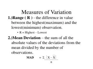
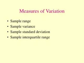
Measures of variation • Variation measures consistency • Range = (highest value - lowest value)/2 • Standard deviation: Precision arrows jungle arrows Same mean length, but different variation!
Measure of variation of all values from mean Positive or zero (data = ) Larger deviations, larger s Can increase dramatically with outliers Same units as original data values Recipe: Compute the mean Substract mean from Individual values Square the differences Add the squared differences Divide by n-1. Take the square root. Example: waiting times Bank Consistency 6 5 4 4 6 5 Bank Unpredictable 0 15 5 0 0 10 Mean: (6+5+4+4+6+5)/6=5 (6-5)=1,(5-5)=0, (4-5)=-1, (4-5)=-1, (6-5)=1, 0 12=1 , 02=0, (-1)2=1, (-1)2=1, 12=1,02=0 ∑ 1+0+1+1+1+0 = 4 n-1=6-1=5 4/5=0.8 √0.8 = 0.9 min vs 6.3 min Standard deviation
Example using fast formula: Find values of n, , n=6 6 values in sample = 30 adding the values = 62+52+42 +42 +52+ 62= 154 Standard deviation of a population divide by N - mu (population mean) Sigma (st. dev. of population) Different notations in calculators Excell: STDEVP instead of STDEV Standard deviation of sample and population Estimating s and : (highest value - lowest value)/4
A statistics class of 20 students obtains the following grades: To rapidly approximate the mean, we take a random sample of 5 students. At random, we pick x= (78+92+64+83+78)/5=395/5 =79 s =√((78-79) 2 +(92-79) 2 +(64-79)2+(83-79) 2 +(78-79)2)/4 =√(( -1) 2 + ( 13 ) 2 + ( -15 )2+ ( 4 ) 2 +( -1 )2)/4 =√( 1 + 169 + 225 + 16 + 1)/4 =√( 412)/4 =√( 103) = 10.15 The population mean is obtained by adding all grades and dividing by 20, which is 79.95. The population variance is 10.71. Which we can obtain using Excell: Example: class grades
Variance Variance = square of standard deviation sample population General terms refering to variation: dispersion, spread, variation Variance: specific definition Ex: finding a variance 0.8, 40 Examples: In class grade case, sample standard deviation was 10.15. Therefore, s2=103. The population standard deviation was 10.71, therefore, 2=10.71 2= 114.7. Variance and coefficient of variation
Coefficient of variation allows to compare dispersion of completely different data sets ex: consistent bank data set 6,5,4,4,6,5; x=5, s=0.9 CV=.9/5=0.18 Class sample: x=79, s=10.1 CV=10.1/79=0.13 Variation of consistent bank is larger than that of the class in relative terms! Coefficient of variation CV [p.155 ex. 49] Describes the standard deviation relative to the mean: Coefficient of variation In previous example, CVsample=10.1/79 =12.8% CVpopulation=10.71/ 79.95 =13.4%
Why use variance, standard deviation is more intuitive? (Independent) variances have additive properties Probabilistic properties Standard deviation is more intuitive Why divide sample st. dev by n-1? Only n-1 free parameters Empirical rule for data with normal distribution 68% of data 95% of data 99.7% of data More on variance and standard deviation Example: Adult IQ scores have a bell-shaped distribution with mean of 100 and a standard deviation of 15. What percentage of adults have IQ in 55:145 range? s=15, 3s=45, x-3s=55, x+3s=145 Hence, 99.7% of adults have IQs in that range. Chebyshev’s theorem: At least 1-1/k2 percent of the data lie between k standard deviations from the mean. Ex: At least 1-1/3^2=8/9=89% of the data lie within 3 st. dev. of the mean.
The mean and the median are often different • This difference gives us clues about the shape of the distribution • Is it symmetric? • Is it skewed left? • Is it skewed right? • Are there any extreme values?
Symmetric – the mean will usually be close to the median • Skewed left – the mean will usually be smaller than the median • Skewed right – the mean will usually be larger than the median • Skewness: Pearson’s index I=3( mean-median )/s • If I < -1 or I > 1: significantly skewed
For a mostly symmetric distribution, the mean and the median will be roughly equal • Many variables, such as birth weights below, are approximately symmetric
Summary: Chapter 3 – Sections 1and 2 • Mean • The center of gravity • Useful for roughly symmetric quantitative data • Median • Splits the data into halves • Useful for highly skewed quantitative data • Mode • The most frequent value • Useful for qualitative data • Range • The maximum minus the minimum • Not a resistant measurement • Variance and standard deviation • Measures deviations from the mean • Not a resistant measurement • Empirical rule • About 68% of the data is within 1 standard deviation • About 95% of the data is within 2 standard deviations
Summary: Chapter 3 – Section 3 (Grouped Data) • As an example, for the following frequency table, we calculate the mean as if • The value 1 occurred 3 times • The value 3 occurred 7 times • The value 5 occurred 6 times • The value 7 occurred 1 time
Evaluating this formula • The mean is about 3.6 • In mathematical notation • This would be μ for the population mean and for the sample mean
Finding s from a frequency distribution Interpreting a known value of the standard deviation s: If the standard deviation s is known, use it to find rough estimates of the minimum and maximum “usual” sample values by using max “usual” value ≈ mean + 2(st. dev) min “usual” value ≈ mean - 2(st. dev) Variance and Standard deviation (grouped data) Example: cotinine levels of smokers N-1: DATA 3,6,9 =6, 2=6 Samples (replacement): 33 36 39 63 66 69 93 96 99 x = 3 4.5 6 4.5 6 7.5 6 7.5 9 ∑(x-x )2 = 0 4.5 18 4.5 0 4.5 18 4.5 0 S2=(divide by n-1=2-1) 0 4.5 18 4.5 0 4.5 18 4.5 0 Mean value of s2=54/9 = 6 S2=(divide by n=2)0 2.25 9 2.25 0 2.25 9 2.25 0 Mean value of s2=27/9 = 3 using Excel we obtain with which we calculate:
Useful for comparing different data sets z scores Number of standard deviations that a value x is above of below the mean Percentiles: Percentile of value x Px sample population number of values less than x Px= total number of values Measures of relative standing Example data point 48 in Smoker data 8/40*100=20th percentile = P20 Exercise: Locate the percentiles of data points 1, 130 and 250. Example: • NBA Jordan 78, =69, =2.8 • WNBA Lobo 76, =63.6, =2.5 Number of standard deviations that a value x is above of below the mean • J: z=(x-)/=(78-69)/2.8=3.21 • L: z=(x-)/=(76-63.6)/2.5=4.96
Conversely, if you are looking for data in the kth percentile: L=(k/100)*n n total number of values k percentiles being used L locator that gives position of a value (the 12th value in the sorted list L=12) Pk kth percentile (ex: P25 is 25th percentile) Quartiles: Q1,= P25, Q2 = P50 =median, Q3= P75 START number of values less than x Pk: k= SORT DATA total number of values Compute L=(k/100)*n n=number of values k=percentile Yes: L whole number? take average of Lth and (L+1)st value as Pk No: ROUND UP Pk is the Lth value Percentiles and Quartiles Pk: k = (L – 1)/n •100 Example: data point 48 in Smoker data is 9th on table, n= 40. (9 – 1)/40 •100=20 48 is in P20 or 20th percentile or the first quartile Q1. Data point 234 is 28th. k=(28 – 1)/40 •100= 68th percentile, or the 3rd quartile Q3. Example: In class table ( n = 20 ) • find value of 21 percentile • L=21/100 * 20 = 4.2 • round up to 5th data point • --> P21 = 71 • find the 80th percentile: • L=80/100 * 20 = 16, • WHOLE NUMBER: • P80 =(89+92)/2=90.5
Exploratory data analysis is the process of using statistical tools (graphs, measures of center and variation) to investigate data sets in order to understand their characteristics. Box plots have less information than histograms and stem-and-leaf plots Not that often used with only one set of data Good when comparing many different sets of data Exploratory Data Analysis Outlier: Extreme value. (often they are typos when collecting data, but not always). • can have a dramatic effect on mean • can have dr. effect on standard deviation • … on histogram